Overview & Introduction

DA101: R scripting

1 Introductory stuff

You can reach us at david.eubanks@furman.edu and scott.moore9@furman.edu.
The course web site is rforir.netlify.app. (It will soon be easier to remember: rforir.com. But not quite yet.)

1.1 The Why of the Class

Help you improve your ability to work with data, thereby

Becoming more efficient and more effective at your jobs, and
Helping others make better decisions.

But, really… Viva la revolución!

The real point of this class is to overthrow the hegemony of spreadsheet-based analyses, to spread a new way of working that enables repeatable analyses, one that has the inherent capacity to enable more efficient workflows while at the same time minimizing the amount of busy-work and boring, repetitive tasks that have to be done.

1.2 Class Goals

Demonstrate the superiority of generating analyses with R/tidyverse scripting to the use of spreadsheets
Describe a unifying high-level process for analyzing data using R
Demonstrate how to use RStudio to develop, test, and execute automated data processes
Demonstrate the basic commands from the R/tidyverse package that replicate (and improve on) common spreadsheet operations

By the end of this course, you will generally be familiar with R and RStudio and the tidyverse, how to write and run R scripts, and how to do analysis using all of these tools.

1.3 Introductions

Instructors
- Dr. David Eubanks (david.eubanks@furman.edu)
- Dr. Scott Moore (scott.moore9@furman.edu)
Participants
- Holy Cross, Northeast Ohio Medical University, Kean University, WVU/Parkersburg, Furman, UTennessee System, UTexas/Dallas, Texas Tech, Ketchum University, Hope College
- If you’d like (and haven’t already), write your name, job title, and contact info in the chat. We’ll distribute it afterwards.

If you send either of us an email related to this class, please put “DA101” at the beginning of the subject line. Thanks.

1.4 Class schedule

Wk #	Mon 3-4:30pmET	Wed 3-4pmET
1	2/3: Overview & basics	2/5: Prob sess
2	2/10: Summary stats & Pivoting	2/12: Prob sess
x	2/17: NO CLASS	2/19: NO CLASS
3	2/24: Joining tables	2/26: Prob sess
4	3/3: Putting it all together	3/5: Prob sess
x	3/10: NO CLASS	3/12: NO CLASS
5	3/17: Final project presentations	CLASS OVER

We will make the link to the Monday class recording available after the class concludes (probably the next day since it takes a while for it to be processed by Zoom).

1.5 The How of this class

You are learning a language
As such, you have to speak that language as often as possible!
We are giving you lots of opportunities to do so
You will get better at working in R in proportion to the amount of time you spend on it

1.6 Weekly sessions

Monday class:
- Introduced to topics
- In-class group work
- Ask questions

Wednesday class
- Problem sessions (no lecture)
- Just lets you work through exercises
- Your questions will drive what we do during this time. Ask about the lessons, exercises, projects, or anything related to the class.

The problem sessions were recommended by last year’s class.

1.7 Assignments each week

Lessons: either web-based or in RStudio (example)
Reading: read through and reference appropriate pages on rforir.com.
Homework: either web-based or in RStudio (example)
Personal project: each week, progressively refine your project (heavily weighted towards end of course)
Hint: Complete as much of the weekly lessons as possible before Wednesday’s class so that you can work on the homework during the problem session.

You have a whole ecology of learning resources at your disposal in this class:

The lecture-centered class session introduces you to the concepts that you will be focusing on during that week.
After attending the lecture (or watching the recording if you cannot attend), then you should work through the lessons. These consist of a sequence of exercises that you can compete either within a Web page or within RStudio. If you complete them within a Web page, then you will have hints available to you to help you complete them successfully.
While you are working through the lessons, you may also find it beneficial to read some of the resources available on the course’s accompanying Web site, rforir. This Web site acts as the course’s “textbook”.
After completing the lessons (or, at least, as many as you can), you should come to the problem session and begin to work through the homework. Both the professors and the other students will all be there to ask questions of when you are, inevitably, stymied.
Again, you can complete the homeworks either within a Web page or within RStudio. In addition to the hints that were similarly available within the lessons, your submission to each question will be assessed by a automated grader and try to give you feedback appropriate to the problem you appear to be having.
Finally, the personal project will be where the whole course comes together for you. You should find a project that you currently do for your job and complete it using the skills that you have used in this course. This is what you will turn in to us at the end of class.

2 Automated Institutional Research

2.1 The whole data science process

This is the process we’ll take you through in our courses
- In this class, we focus on Import, Tidy, Transform, and a bit on Model
Today we’ll provide an overview of the whole thing

We will cover the tidyverse’s graphing capabilities (housed in ggplot2) in DA102 and R’s reporting capabilities (housed in quarto) in DA103.

2.2 Benefits of `R` over `Excel`

Much more efficient
Greater ability to work with large data sets
Iterative at its core
Better graphics

Create better & more complete reports
- Better structured
- More repeatable
- More informative
R is free and open source

A short article on this topic can be found here.

3 Your final report: Working with `R`

3.1 Your course project

On the last day of the class, each of you will share your project with the other students
Data types and structures
Scripting in R
Tools built into R (including the tidyverse)
Exploring data
Generating reports by filtering, selecting, arranging, and summarizing

3.2 Student discussion: Types of reports

Address the questions:
- What types of reports do you work on in your job?
- How do you currently do that work?
- How much time could be saved by avoiding repetitive work?
Discuss in your group
Then we’ll discuss as a class

4 Working with `R`, `RStudio`, & the `tidyverse`

4.1 How these pieces fit together

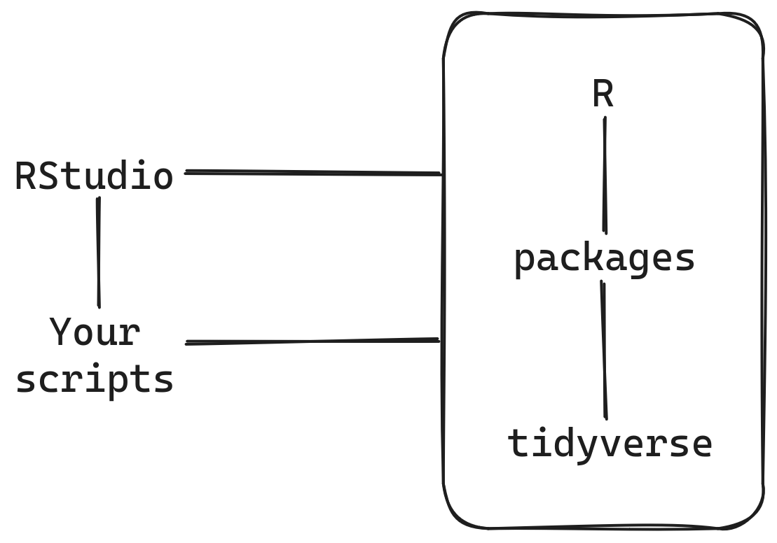
R was created back in August 1993 by two professors in New Zealand.
RStudio is an integrated development environment from Posit that has been in development since 2010.
Packages are user-defined, contributed, and managed software that are the means by which functionality is added to R. There are at least 16,000 packages are available.
The tidyverse is an extensive (and revolutionary) set of packages introduced by Hadley Wickham beginning in 2007.

4.2 What we’re going to show right now

Importing data
Exploring the data
Selecting/displaying data
Sorting data
Choosing data
Summarizing data

I am going to demonstrate within RStudio
You can go back and re-create it using this page
You can also re-create it within RStudio using the week1-files project that you have already downloaded

4.3 In-class collaboration

Follow this trail:

On rforir.netlify.app, click on the Class home page
Go down to Section 4 “Schedule for the course”
In 4.1.1, look under Resources
Look under “In class”
Click on In-class collaboration document
Follow the instructions while working with each other

https://rforir.netlify.app/rapp-wasm/data-analysis/da101/2025-02/week1-collaborate.html

5 Before next week’s class

5.1 Your to-do list

What you’ll be doing this week

Work on this week’s lessons
Come to Wednesday’s problem session ready to work on this week’s homework (preferably) or lessons
Complete this week’s homework before next Monday
Start thinking about your own project

6 Another demonstrate project (not covered in class)

6.1 Importing data

Bring the data into R so that it can be manipulated
CSV is the file format that we will use.

term <- read_csv("data/term.csv")

Rows: 28 Columns: 4
── Column specification ────────────────────────────────────────────────────────
Delimiter: ","
chr (2): Season, SchoolYear
dbl (2): TermID, CalendarYear

ℹ Use `spec()` to retrieve the full column specification for this data.
ℹ Specify the column types or set `show_col_types = FALSE` to quiet this message.

R can import data from all kinds of places — CSV files, Excel files, and databases of all types.

6.2 Learn about the data: `summary()`

summary() gives an overview of the columns

summary(term)

     TermID         Season           CalendarYear   SchoolYear       
 Min.   :101.0   Length:28          Min.   :2009   Length:28         
 1st Qu.:107.8   Class :character   1st Qu.:2013   Class :character  
 Median :114.5   Mode  :character   Median :2016   Mode  :character  
 Mean   :114.5                      Mean   :2016                     
 3rd Qu.:121.2                      3rd Qu.:2019                     
 Max.   :128.0                      Max.   :2023

This tells us that the data frame has four columns, and it gives us a bit of information about each.

6.3 Look at the data (`RStudio`): `view()`

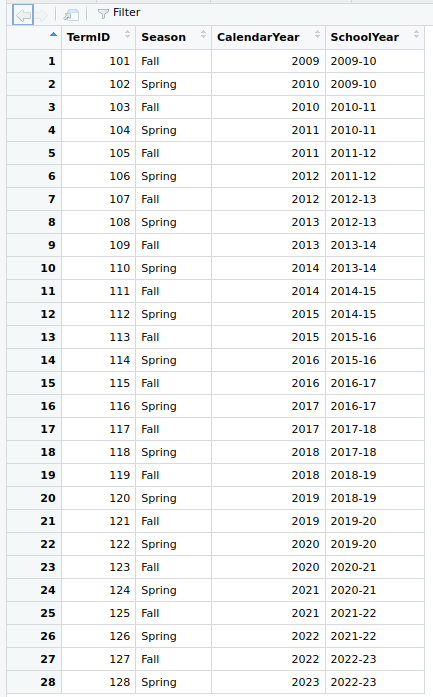
view() shows you the data in a spreadsheet format

view(term)

This should seem familiar to those who work in a spreadsheet program.

6.4 Look at the data: `head()`

head() shows the first few rows of the data

head(term)

# A tibble: 6 × 4
  TermID Season CalendarYear SchoolYear
   <dbl> <chr>         <dbl> <chr>     
1    101 Fall           2009 2009-10   
2    102 Spring         2010 2009-10   
3    103 Fall           2010 2010-11   
4    104 Spring         2011 2010-11   
5    105 Fall           2011 2011-12   
6    106 Spring         2012 2011-12

Given that data frames can have millions of rows, it can be quite convenient to have a tool that makes it so easy to just look at a bit of data.

6.5 The Pipe (`|>`)

An alternate, preferred way to construct R commands
The left side is fed into (piped into) the right side, and is used as the first argument to that command.

term |>
  head()

# A tibble: 6 × 4
  TermID Season CalendarYear SchoolYear
   <dbl> <chr>         <dbl> <chr>     
1    101 Fall           2009 2009-10   
2    102 Spring         2010 2009-10   
3    103 Fall           2010 2010-11   
4    104 Spring         2011 2010-11   
5    105 Fall           2011 2011-12   
6    106 Spring         2012 2011-12

The ability to program in this way (or, equivalently, to write scripts this way) is the motivating factor behind the creation of the whole tidyverse. Many people find it much more approachable than traditional, functional-based methods.

6.6 Select certain columns: `select()`

Choose which columns to print or work with.

term |>
  select(TermID, Season, CalendarYear)

select: dropped one variable (SchoolYear)

# A tibble: 28 × 3
   TermID Season CalendarYear
    <dbl> <chr>         <dbl>
 1    101 Fall           2009
 2    102 Spring         2010
 3    103 Fall           2010
 4    104 Spring         2011
 5    105 Fall           2011
 6    106 Spring         2012
 7    107 Fall           2012
 8    108 Spring         2013
 9    109 Fall           2013
10    110 Spring         2014
# ℹ 18 more rows

This command says “Given the term data frame, display three columns (TermID, Season, and CalendarYear).”

6.7 Select the unique/distinct values from columns: `distinct()`

term |> 
  distinct(Season)

distinct: removed 26 rows (93%), 2 rows remaining

# A tibble: 2 × 1
  Season
  <chr> 
1 Fall  
2 Spring

term |>
  select(Season)

select: dropped 3 variables (TermID, CalendarYear, SchoolYear)

# A tibble: 28 × 1
   Season
   <chr> 
 1 Fall  
 2 Spring
 3 Fall  
 4 Spring
 5 Fall  
 6 Spring
 7 Fall  
 8 Spring
 9 Fall  
10 Spring
# ℹ 18 more rows

The distinct() operator tells tidyverse to look through all of the rows and find the unique values found in all of them.

6.8 Sort by column(s): `arrange()`

Specify in what order to print the rows.

term |>
  select(TermID, Season, CalendarYear) |>
  arrange(desc(TermID))

select: dropped one variable (SchoolYear)

# A tibble: 28 × 3
   TermID Season CalendarYear
    <dbl> <chr>         <dbl>
 1    128 Spring         2023
 2    127 Fall           2022
 3    126 Spring         2022
 4    125 Fall           2021
 5    124 Spring         2021
 6    123 Fall           2020
 7    122 Spring         2020
 8    121 Fall           2019
 9    120 Spring         2019
10    119 Fall           2018
# ℹ 18 more rows

Be sure to understand how the pipe operator works in this command. Read it from top-to-bottom:

Send the term data frame to the next statement.
Select these three columns from the whole term data frame.
Sort these three columns from the whole term data frame (since that is what was given to this command) by the TermID column (but in descending order).

6.9 Select certain rows 1/2: `filter()`

Select which rows to print or work with.

term |>
  select(TermID, Season, CalendarYear) |>
  arrange(TermID) |>
  filter(Season == "Fall")

select: dropped one variable (SchoolYear)
filter: removed 14 rows (50%), 14 rows remaining

# A tibble: 14 × 3
   TermID Season CalendarYear
    <dbl> <chr>         <dbl>
 1    101 Fall           2009
 2    103 Fall           2010
 3    105 Fall           2011
 4    107 Fall           2012
 5    109 Fall           2013
 6    111 Fall           2014
 7    113 Fall           2015
 8    115 Fall           2016
 9    117 Fall           2017
10    119 Fall           2018
11    121 Fall           2019
12    123 Fall           2020
13    125 Fall           2021
14    127 Fall           2022

Again, realize that the input into the filter() command is the output of the arrange() command — which is the three columns of the term data frame sorted by TermID.

The filter() command tells the tidyverse to filter to include only those rows for which Season is equal to "Fall" (that is, a capital F followed by a lower-case `all).

6.10 Select certain rows 2/2: `filter()`

term |>
  select(TermID, Season, CalendarYear) |>
  arrange(TermID) |>
  filter(Season == "Fall",
         CalendarYear >= 2019)

select: dropped one variable (SchoolYear)
filter: removed 24 rows (86%), 4 rows remaining

# A tibble: 4 × 3
  TermID Season CalendarYear
   <dbl> <chr>         <dbl>
1    121 Fall           2019
2    123 Fall           2020
3    125 Fall           2021
4    127 Fall           2022

asdf

6.11 Summarizing: `group_by()` & `summarize()`

Specify how to and which summary statistics to calculate.

term |>
  select(SchoolYear) |>
  group_by(SchoolYear) |>
  summarize(Count = n()) |>
  head(5)

select: dropped 3 variables (TermID, Season, CalendarYear)
group_by: one grouping variable (SchoolYear)
summarize: now 14 rows and 2 columns, ungrouped

# A tibble: 5 × 2
  SchoolYear Count
  <chr>      <int>
1 2009-10        2
2 2010-11        2
3 2011-12        2
4 2012-13        2
5 2013-14        2

Let’s go through what this whole series of commands is doing:

Start with the whole term data frame.
Select just the SchoolYear column.
For the whole SchoolYear column of the term data frame, group all of the rows by the SchoolYear value.
In a new Count column, put the value of the number of rows that have the same SchoolYear value (since that’s what it was grouped by).
Display just the first five rows.