Joins

In this page, we’re going to be focusing on joins, a new kind of operation for many of you. It is the one, single thing that enables all of this work in R both to be possible and to be challenging mentally.

Joins refer to the action of linking two or more tables together in a way that facilitates analysis. The separation of data into separate tables (in the first place) enables a more logical and consistent structuring of data that is, in turn, easier both to access and to maintain.

1 Our data

In this collection of data, we have 5 students, 5 jobs, and 5 clubs. The employment data frame shows the two students who each have two jobs. The `membership data frame shows the three students who are members of clubs (one is a member of two of them).

A feature of this organization of data is that every separate data frame is about one thing, and one thing only.

students <-
  tibble(id = 1:5,
         given_name = c("Al", "Bob", "Charles", 
                        "Dave", "Ed"),
         family_name = c("Adams", "Barker", "Cook", 
                         "Davidson", "Edwards"))
jobs <-
  tibble(id = 1:5,
         title = c("Analyst", "Baker", "Cook", 
                   "Dog Catcher", "Evangelist"))
clubs <-
  tibble(id = 1:5,
         title = c("Archery", "Badminton", "Chess", 
                   "Dahlias", "Eating"))
employment <-
  tibble(student = c(1, 1, 2, 2),
         job = c(1, 3, 3, 4))
membership <-
  tibble(student = c(2, 2, 3, 5),
         club = c(1, 4, 4, 5))

2 Concept: Keys

Keys are central to a data set’s ability to represent relationships between tables. Let’s get a better understanding here.

2.1 Primary Keys

A primary key is a column (or set of columns) whose value can be used to identify one-and-only-one row in that data frame. Satisfy yourself that each of the following primary keys uniquely identifies one-and-only-one row in its data frame.

[students.id]
[jobs.id]
[clubs.id]
employment.[student, job]
membership.[student, club]

2.2 Foreign Keys

A foreign key is a column (or set of columns) whose value can be used to identify one-and-only-one row in another data frame. It must be the primary key in that other data frame. The foreign keys in this example are as follows:

employment.student to students.id
employment.job to jobs.id
membership.student to students.id
membership.club to clubs.id

Each single foreign key value refers to one-and-only-one primary key value. However, sometimes one particular primary key value can refer to many different rows where it is embedded as a foreign key. (Make sure you understand how these two sentences differ and why they don’t contradict each other!)

2.3 Explore your understanding

What if you wanted to add some new pieces of data to this set of data. Where would you put the following columns:

Date that a club was founded
Date that a student joined a club
Date that a student began working at a job
Possible pay range for a particular job

The answers to these questions can be determined by thinking about what specific primary key would determine the value of each of the above.

Here are my answers:

Date that a club was founded: Put founding_date into clubs. Each club can have one and only one founding date.
Date that a student joined a club: Put join_date into membership. Each student can join a specific club just one time.
Date that a student began working at a job: Put start_date into employment. Each student can start a specific job on just one date.
Possible pay range for a particular job: Put min_pay_rate and max_pay_rate into jobs. Each job can have one and only one pay range, but that pay range is defined by two values (a minimum and a maximum). Each column should contain one and only one value.

3 Entity-Relationship (ER) diagram

An entity-relationship diagram is a graphical tool for representing relationships (that is, foreign keys). The entities are the boxes. The relationships are the lines. (By the way, there are many ways to draw ER diagrams, and this is just one of them. They all generally work, and the most important thing is to simply choose one of them in your organization.)

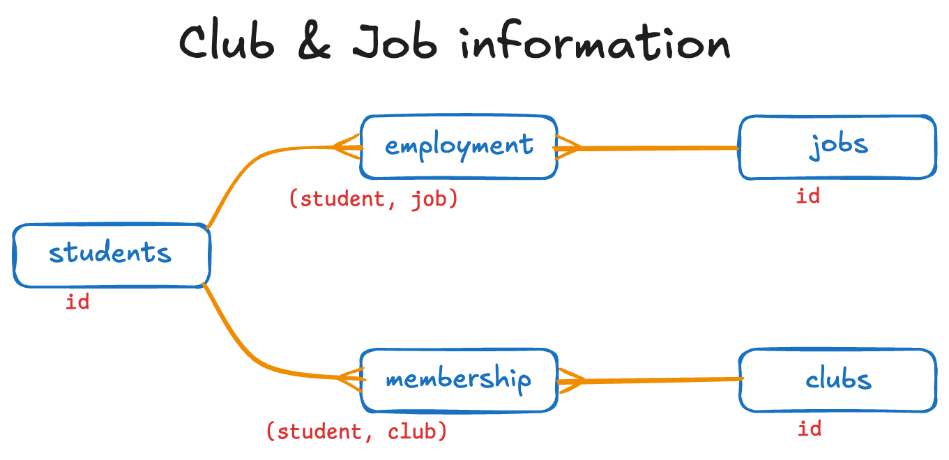
You read the relationship with the following structure, starting at the single (line) end and moving to the multiple (fork) end:

For every LINE, there can be many FORK. For any single FORK, there can be at most one LINE.

Thus, we have the following represented in this diagram:

For every student, there can be many employments.
For every employment, there is one and only one job.
For every job, there can be many employments.
For every employment, there is one and only one job.
For every student, there can be many memberships.
For every membership, there can be one and only one club.
For every club, there can be many memberships.
For every membership, there can be one and only one student.

The red text below each entity is the primary key. You should find a foreign key in the FORK END that refers to the primary key at the LINE END.

4 Joins and Primary and Foreign Keys

Joins are the way that the R/tidyverse brings together (joins!) data from multiple data frames. Primary and foreign keys within the data are what enables this to work. (This concept is applicable in all databases (since the 1970s). These are called relational databases.)

This is also applicable to all analytic software (e.g., R, Tableau, etc.). And this is so much faster than vlookup() from Excel. It’s built-in to databases rather than being an add-on.

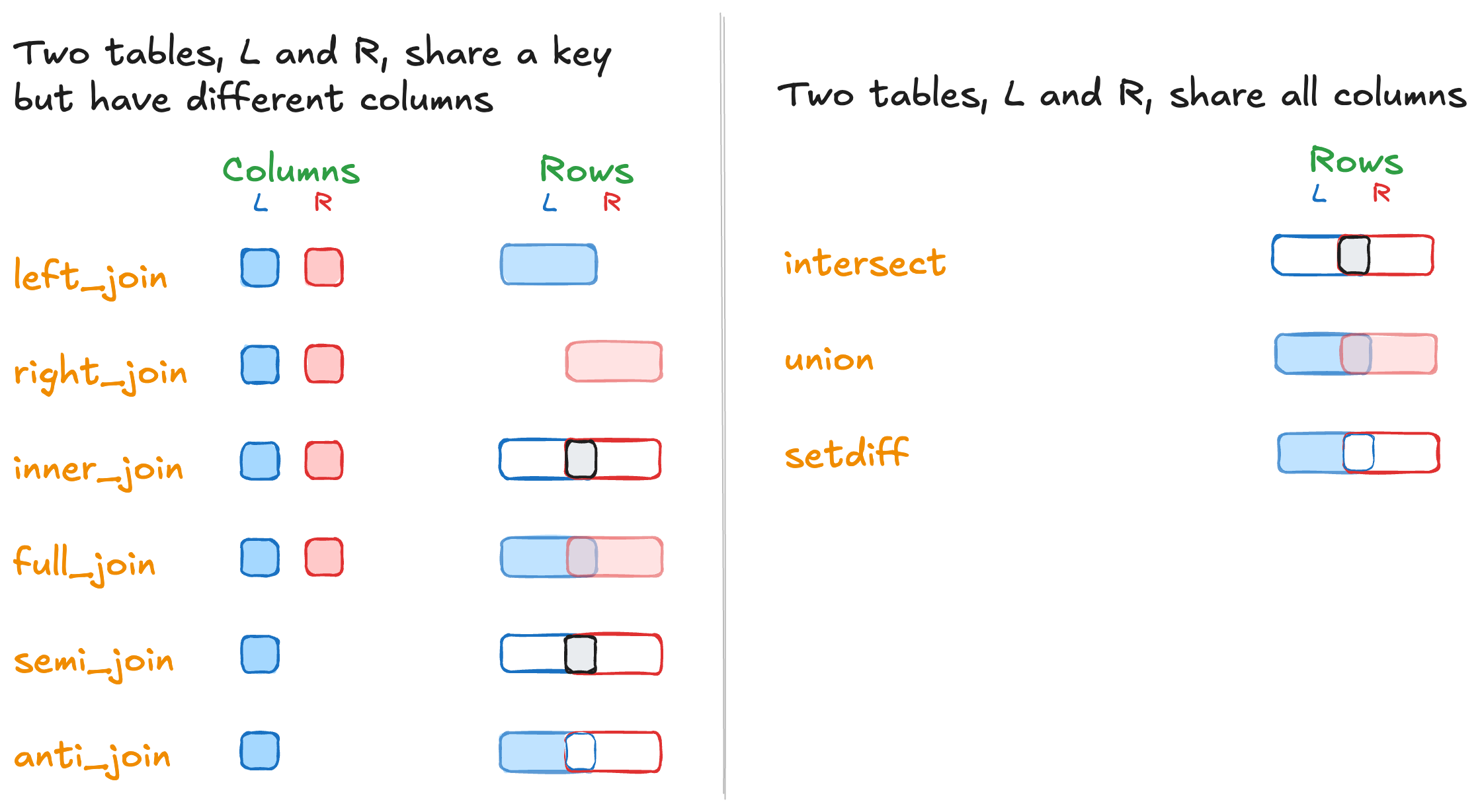
R/tidyverse has six kinds of joins. The following captures the options for joining tables together:

5 `left_join()`: the workhorse

If you understand how to use this join, then the rest will be straight-forward to use. You can get by using just this type of join for most of your work.

Description: All info from left plus possible matches with right
Rows included: all from left
Columns included: all from left and all from right (with NAs when no match is found)

5.1 Template

LEFT_DF |> 
  left_join(RIGHT_DF, 
            join_by(LEFTKEY == RIGHTKEY))

5.2 Example 1

The question: List all students with the club names, if any, that they belong to.

students |>
  left_join(membership, join_by(id == student)) |>
  left_join(clubs, join_by(club == id))

We’re traversing in the ER diagram starting at student and going down a fork and then up a line (from students to membership to clubs). Note that the columns going across are in order by when they were encountered. club is picked up from membership (but not student since it is replicated by id which is already there) and then title is picked up from clubs (but not id since it is replicated by club which is already there).

When specifying the join_by() columns, we ensure that we are including the whole and correct primary and foreign keys.

5.3 Example 2

The question: List all students with the club names, if any, that they belong to.

students |>
  left_join(membership, join_by(id == student)) |>
  left_join(clubs, join_by(club == id)) |>
  mutate(full_name = str_c(given_name, " ", family_name)) |>
  select(full_name, title)

The question here is the same, so this query starts out the same as the previous query. The difference is that this time we have chosen to list just the student’s full name and the title of the club.

The str_c() function concatenates the three text strings and puts the result in the new full_name column. The select() statement directs the R/tidyverse to display just two columns.

6 Aside: `join_by()`

You have three options for specifying how the two data frames are to be joined:

join_by(LEFTKEY == RIGHTKEY): Is always appropriate.
join_by(KEYNAME): When the LEFTKEY and RIGHTKEY are named the same.
nothing at all: When the LEFTKEY and RIGHTKEY are named the same and are the only two columns in the two data frames that have the same names.
- This one makes us nervous because it can fail without giving an error. Don’t use it.

7 `right_join()`

Description: All info from right plus possible matches with left
Rows included: all from right
Columns included: all from right and all from left (with NAs when no match is found)

7.1 Template

LEFT_DF |> 
  right_join(RIGHT_DF, 
             join_by(LEFTKEY == RIGHTKEY))

7.2 Example

The question: List the student names and job titles for only students with jobs.

We’re doing this in three stages.

7.2.1 Stage 1

students |>
  right_join(employment, join_by(id == student)) |>
  kbl() |> kable_minimal()

id	given_name	family_name	job
1	Al	Adams	1
1	Al	Adams	3
2	Bob	Barker	3
2	Bob	Barker	4

In this first stage, we want to complete the first join. We choose a right join so that we have all the information from students but only for those students who have a job (i.e., they are in the employment data frame).

7.2.2 Stage 2

students |>
  right_join(employment, join_by(id == student)) |>
  left_join(jobs, join_by(job == id)) |>
  kbl() |> kable_minimal()

id	given_name	family_name	job	title
1	Al	Adams	1	Analyst
1	Al	Adams	3	Cook
2	Bob	Barker	3	Cook
2	Bob	Barker	4	Dog Catcher

In this second stage, we complete the second join. We use a left_join() because every row in employment will have an associated row in the jobs data frame (since jobs.job is never empty).

7.2.3 Stage 3

students |>
  right_join(employment, join_by(id == student)) |>
  left_join(jobs, join_by(job == id)) |>
  mutate(full_name = str_c(given_name, 
                           family_name, 
                           sep = " ")) |>
  select("Full name" = full_name, 
         "Job title" = title) |>
  kbl() |> 
  kable_minimal()

Full name	Job title
Al Adams	Analyst
Al Adams	Cook
Bob Barker	Cook
Bob Barker	Dog Catcher

In this third stage, we improve the formatting of the name and the column headers.

8 `inner_join()`

Description: All info from right and left but only when there is a match
Rows included: only those rows when there is a match
Columns included: all from right and all from left

8.1 Template

LEFT_DF |> 
  inner_join(RIGHT_DF, 
             join_by(LEFTKEY == RIGHTKEY))

Note: The following examples have many twists and turns. You might think that these are because of the complexity of inner_join() itself. Wrong. It’s because of the operations of the general join facility.

8.2 Example 1

The question: How many students have both a job and membership in a club?

8.2.1 Version 1

In this version we are going to traverse the ER diagram as we have been doing: table by table.

8.2.1.1 Version 1: Step 1

In this first step, we are going to simply attempt to join along the relationships between the tables.

The first inner_join() joins employment to students. Since the values in student are equivalent to the id column in students, R has a rule to always keep just the first column listed (in this case, student from employment).

The second inner_join() joins the result of the first join to membership by the student column in each. Again, by R’s rule, it keeps just one of the student columns.

employment |>
  inner_join(students, join_by(student == id)) |>
  inner_join(membership, join_by(student))

Warning in inner_join(inner_join(employment, students, join_by(student == : Detected an unexpected many-to-many relationship between `x` and `y`.
ℹ Row 3 of `x` matches multiple rows in `y`.
ℹ Row 1 of `y` matches multiple rows in `x`.
ℹ If a many-to-many relationship is expected, set `relationship =
  "many-to-many"` to silence this warning.

I’m sure that you can’t miss this very long warning given by the tidyverse. It tells us that we have a many-to-many relationship between rows in employment (the far left data frame) and membership (the far right data frame) — that is, tidyverse has detected that a student in employment can be in more than one row in membership, and that a student in membership can be in more than one row in employment. This is, in formal database nomenclature, a many-to-many relationship. There’s nothing wrong with this! It’s just a special case that it wants you to be know exists.

The warning message gives a very useful hint as to how to silence this warning at the end of the message. We’ll try it in the next step.

8.2.1.2 Version 1: Step 2

Here we add the relationship clause to the second inner_join(). It now gives the same result as the above but without the warning message.

employment |>
  inner_join(students, join_by(student == id)) |>
  inner_join(membership, join_by(student), 
             relationship = "many-to-many")

8.2.1.3 Version 1: Step 3

The original question was to simply calculate the number of students who have both a job and a club membership. So far, we have displayed all of the information about the job and club. Let’s now just answer the question.

employment |>
  inner_join(students, join_by(student == id)) |>
  inner_join(membership, join_by(student), 
             relationship = "many-to-many") |>
  select(student) |>
  n_distinct()

[1] 1

8.2.2 Version 2

In this version, we are going to skip the students table and directly join the employment and membership tables. Why do we think we can do this? Well, first, because we are not going to end up using select() on any columns in the students data frame. Second, because the student column in both the employment and membership tables are foreign keys to the students table. Third, there are no intervening tables that change the meaning of the student column in either of those tables.

8.2.2.1 Attempt 1

In this attempt, we directly join the employment data frame to the membership data frame:

employment |>
  inner_join(membership, join_by(student)) |>
  select(student) |>
  n_distinct()

Warning in inner_join(employment, membership, join_by(student)): Detected an unexpected many-to-many relationship between `x` and `y`.
ℹ Row 3 of `x` matches multiple rows in `y`.
ℹ Row 1 of `y` matches multiple rows in `x`.
ℹ If a many-to-many relationship is expected, set `relationship =
  "many-to-many"` to silence this warning.

[1] 1

As in attempt 1, we get the warning from tidyverse; let’s fix that.

8.2.2.2 Attempt 2

Here, there is just the one inner_join(), so we put the relationship clause in it:

employment |>
  inner_join(membership, join_by(student),
             relationship = "many-to-many") |>
  select(student) |>
  n_distinct()

[1] 1

8.2.3 Version 3

Since an inner_join requires that the key be in both tables (and since all columns from both tables would be included), we could have written the query like this (i.e., in the reverse order to the previous query):

membership |>
  inner_join(employment, join_by(student),
             relationship = "many-to-many") |>
  select(student) |>
  n_distinct()

[1] 1

Both inner_join() and full_join() queries can be done in either order; the meaning of the other join-types change when executed in the reverse order.

8.3 Example 2

The question: List the full names, job titles, and clubs, for only those students who have both a job and membership in a club.

employment |>
  inner_join(membership, join_by(student),
             relationship = "many-to-many") |>
  left_join(students, join_by(student == id)) |>
  left_join(jobs, join_by(job == id)) |>
  left_join(clubs, join_by(club == id)) |>
  mutate(full_name = str_c(family_name, ", ", given_name)) |>
  select(full_name, Job = title.x, Club = title.y)

This time instead of a count we are looking for information about the students, jobs, and clubs. Let’s explain the four joins:

employment |> inner_join(membership, join_by(...), relationship...): Results in a data frame with student, job, club for all of those students who have both a job and membership in a club. We already know (from above) that this is a many-to-many relationship, so we indicate that here as well.
|> left_join(students, join_by(student == id)): We are joining the result of the previous join with students. We are ensuring that the existing student connects to the row in the students data frame for which it matches the id column. The result is a data frame with columns student, job, club, given_name, and family_name. But, again, it is only for those students who have both a job and membership in a club.
|> left_join(jobs, join_by(job == id)): We are joining the result of the previous join with jobs. We are ensuring that the existing job column matches the id (primary key) column of jobs. This adds the title column from jobs to the existing set of columns (but without adding any rows).
|> left_join(clubs, join_by(club == id)): We are joining the result of the previous join with clubs. We are ensuring that the existing club column matches the id (primary key) column of clubs. This adds the title column from clubs to the existing set of columns.

Note carefully the following: Since we added a title column in the third join and in the fourth join, and since column names have to be unique, R/tidyverse renames the columns to title.x and title.y. We could have avoided this by using rename() after the third join but we generally just let the R/tidyverse handle it first and then we clean it up later.

After those four joins, we use mutate() to calculate a new full_name column. We then use select() to both choose the columns that we want to display and also rename both the title columns.

9 `full_join()`

Description: All info from left and right
Rows included: all from left and right
Columns included: all from left (with NAs when no match is found) and all from right (with NAs when no match is found)

9.1 Template

LEFT_DF |> 
  full_join(RIGHT_DF, 
            join_by(LEFTKEY == RIGHTKEY))

9.2 Example 1

The question: List the ids and first and given names for all students who have either a job or club membership.

We are, again, going to approach this example in three stages.

9.2.1 Stage 1

(students_with_jobs_or_clubs <- membership |>
  full_join(employment, join_by(student),
            relationship = "many-to-many") |>
  select(student))

In this first stage, we define a data frame students_with_jobs_or_clubs that contains just the student id (student) for those students who are members of a club or have a job.

9.2.2 Stage 2

students |>
  left_join(students_with_jobs_or_clubs,
            join_by(id == student))

With this query we can get all the information from the students data frame by performing this left_join() from students to the data frame we just created.

9.2.3 Stage 3

students |>
  left_join(membership |>
              full_join(employment, join_by(student),
                        relationship = "many-to-many") |>
              select(student),
            join_by(id == student))

The trick shown here is a little mind-blowing. What’s going on?

The first argument of left_join must be a data frame.
The query membership |> full_join(...) |> select(...) is the same query that we used in part a to define students_with_jobs_or_clubs.
Here we simply substituted the query itself for the name of the data frame that the query was used to create. (Compare them yourselves!)

The R/tidyverse is flexible enough that it can substitute a query for the name of a data table. Who knew?!?

We don’t expect you to use this approach much, but we wanted you to know about it so that you don’t get overly alarmed if you come across it elsewhere.

9.3 Example 2

The question: List the IDs and first and given names for all students who have either a job or club membership.

students |>
  right_join(employment |>
               full_join(membership, join_by(student),
                         relationship = "many-to-many"),
             join_by(id == student)) |> 
  distinct(id, given_name, family_name)

Except for the last line, this query is the same as the last one. The distinct() command enables us to get rid of all of the duplicate students.

10 `anti_join()`

Description: All info from left
Rows included: all from left that are not in right
Columns included: all from left

10.1 Template

LEFT_DF |> 
  anti_join(RIGHT_DF, 
            join_by(LEFTKEY == RIGHTKEY))

10.2 Example 1

The question: List the ids and names of all students who do not have a job.

students |>
  anti_join(employment, join_by(id == student))

The anti_join() is the perfect command for this question. It looks at all the id values in students and chooses only those that are not in the student column of employment. That is, it displays those students who do not have a job! Easy peasy.

10.3 Example 2

The question: List the ids and names of all students and their clubs who are in a club but do not have a job.

membership |>
    anti_join(employment, join_by(student)) |>
    left_join(students, join_by(student == id)) |>
    left_join(clubs, join_by(club == id)) |>
    mutate(full_name = str_c(given_name, " ", family_name)) |>
    select(StID = student, 
           `Full Name` = full_name, 
           Club = title) |>
    kbl() |> kable_minimal()

StID	Full Name	Club
3	Charles Cook	Dahlias
5	Ed Edwards	Eating

By executing an anti_join() from membership to employment, we are choosing those students who are in a club but do not have a job (which is what we wanted).

Now, since we want all the student information, we need to left_join to students. Since every student in membership is in students, we do not have to worry about inserting any NA values.

The third join, a left_join() with clubs, gets us the name of the club (the title column).

We then use mutate() to calculate the full_name column, select() to give three columns more informative names, and then the kable commands to format the table display.

11 `semi_join()`

Description: all info from left but only for those that are also in right
Rows included: all from left that match in right
Columns included: only those from left

11.1 Template

LEFT_DF |> 
  semi_join(RIGHT_DF, 
            join_by(LEFTKEY == RIGHTKEY))

11.2 Example 1

The question: List those students who have jobs.

students |>
    semi_join(employment, join_by(id == student))

This semi_join() statement selects all of the columns from students but only those rows for which students.id is in the student column of employment. That is, it lists all student information for those students who have jobs.

11.3 Example 2

The question: List students who have both jobs and membership in clubs.

students |>
    semi_join(employment, join_by(id == student)) |>
    semi_join(membership, join_by(id == student))

This query starts the same as the previous one. Let’s explain what happens:

students |> semi_join(employment,...): Again, this has selected all student information for those students who have jobs. The result is a data frame with the same columns as are in students but fewer rows (since not all students have jobs).
|> semi_join(membership,...): Now, taking the input from the previous join, this join selects only those rows for students that are members of a club.

After going through both joins, the result is the set of students who have both a job and membership in a club.