grades <- data.frame(
  record_id = 1:1000
) |>
  mutate(
    student_id = sample(1:100, 1000, replace = TRUE),
    section_id = sample(1:50, 1000, replace = TRUE),
    subject = sample(
      c(
        "Biology", "Chemistry",
        "Economics", "Psychology"
      ),
      1000,
      replace = TRUE
    ),
    grade_points = round(4 * rbeta(1000, 5, 1), 1),
    grade_letter = case_when(
      grade_points >= 4.0 ~ "A",
      grade_points >= 3.0 ~ "B",
      grade_points >= 2.0 ~ "C",
      grade_points >= 1.0 ~ "D",
      TRUE ~ "F"
    )
  )
grades <-
  grades |>
  mutate(subject = factor(subject,
    levels = c(
      "Biology", "Chemistry",
      "Economics", "Psychology"
    )
  ))
grades <-
  grades |>
  mutate(grade_letter = factor(grade_letter,
    levels = c("F", "D", "C", "B", "A"),
    ordered = TRUE
))Pivoting Wide to Long to Wide
1 Set up: Create some test data
A data frame is like a table in a database or a spreadsheet. It has rows and named columns. Most of the time, we load data from a file or database. But for a simple example, we can create one like this.
2 The R/tidyverse naturally creates long data
As Excel users know, pivot tables are powerful ways to shape data tables into new forms that include row headers and column headers for the new table that are all chosen from existing columns. For example, we might want to create a college grade report that has each academic subject as a row and each column being a letter grade A through F, with the cell values being the counts or percentages of grades for that subject.
For summary purposes, the easiest way to do this in R/tidyverse is with group_by() and summarize(); see this page on rforir.
For example, to count up letter grades by subject we could use:
Here, count() is a short cut for:
For more information on using count() this way, see this page on rforir.
The result is a “long” data frame, with the two categories we care about,
subjectsandgrade_lettereach represented in a column. For a report, it’s more natural to “pivot” the letter grades to columns.
It is absolutely not the case that you are used to working with data like this unless you have worked with a database. Working with Excel has trained most people to think about data in a wide format.
You need to get comfortable with pivoting data either from long to wide or from wide to long.
3 Widen the data frame with pivot_wider()
Look again at the data output above. What seems weird about this?
More than likely, you expect to see “subject” down the left column and columns from left to right, one for each grade. It’s as if you want one column for each different value in the grade_letter column. File this bit of information away for a moment.
In order to change from the format you see above to the wide format that you might expect to see, you have to pivot the data from long to wide.
We can pick one or more columns that will be used to “widen” the data frame. The values within those columns each become new column headers. For example, as we pointed out above, we could take a grade_letter column with values A through F and create new columns for each of those.
This is the process that you will follow when you want to widen a data frame:
- First select just the columns you want. Pivoting can become complicated and we want to simplify as much as possible. In this case we need
subject(because it will be the left column),grade_letter(because its values will become the column headers), andn(because its values will become the values within the body of the table). - Identify the column that is to be spread out (widened). That is the
names_fromcolumn. - When we spread out the column it creates a lot of new cells. We need to specify what values go in those cells with
values_from. - Do you want to put the column names in order? If so, then set
names_sorttoTRUE.
The following is both an example and provides the general form that you should follow when you need to pivot your own data to a wide format:
grade_counts |>
  select(subject, grade_letter, n) |>
  pivot_wider(
    names_from = grade_letter, # which column to widen
    values_from = n, # what to put in the new cells
    names_sort = TRUE
  ) # put the new cols in order
Go back and carefully review the differences between the original
grade_countsdata frame and this wider format. It is crucial for you to understand what precisely has happened.
4 Custom display function
Pivot tables use a variety of summary statistics in the cells. Here we might want to include the percentage of each grade letter for each subject. A useful trick here is to create a custom display function.
The following code will display counts out of totals, with percentage:
Specifically, what does this do?
- For a given input
nandtotal, it will displayn/totaland then the actual value of the calculation as a percentage. - It uses the
str_c()function to concatenate (join together) a whole series of values, with the result being a string.
Try it out:
Did it do what you expected?
5 Using a custom display function
We are now going to apply the above function to the counts before pivoting; the basic information being pivoted is the same but the format of the results will make it appear different.
This is relatively complicated, and we wouldn’t expect you go come up with this approach on your own. Let’s take a moment to talk through these steps.
grade_counts: we’re working with this data frame.group_by(subject): as before, we are grouping bysubject.mutate(total = sum(n)): we are calculating (usingmutate()and notsummarize()) the total number of grades by subject. How doesRknow to calculate by subject? Because thegroup_by()comes before the calculation.mutate(cell = cell_fmt(n, total)): now we can see why we had to calculatetotalon the previous line — it is needed so that we can pass it to thecell_fmt()function.select(-n, -total): now that we are done withnandtotal, we can remove them from the data frame.pivot_wider(...): the only thing we have changed here is that the information printed within the table itself (that is, thevalues_from) is nowcellthat we just calculated.
grade_counts |>
  group_by(subject) |>
  mutate(
    total = sum(n),
    cell = cell_fmt(n, total)
  ) |>
  select(-n, -total) |> # don't need these cols now
  pivot_wider(
    names_from = grade_letter,
    values_from = cell,
    names_sort = TRUE
  )
More advanced uses of pivot_wider() allow us to pivot multiple columns at once, and to create new column names from the values of each of these. You can find examples in the documentation online. Within rforir.com, look in the left column under “Converting wide to long” for some discussion about this process.
6 Pivot the data frame from wide to long
While above we looked at converting long data to wide data, sometimes we are given wide data and we want to use R to manipulate it. This calls for long data and, to get that, we need to pivot from wide to long.
A common case is with survey data. The following code simulates a survey with 5 questions, each with a 1-5 rating:
survey <- data.frame(record_id = 1:100) |>
  mutate(
    q1 = sample(1:5, 100,
      replace = TRUE,
      p = c(0.1, 0.2, 0.3, 0.2, 0.2)
    ),
    q2 = sample(1:5, 100,
      replace = TRUE,
      p = c(0.2, 0.2, 0.2, 0.2, 0.5)
    ),
    q3 = sample(1:5, 100,
      replace = TRUE,
      p = c(0.2, 0.2, 0.2, 0.2, 0.4)
    ),
    q4 = sample(1:5, 100,
      replace = TRUE,
      p = c(0.05, 0.1, 0.1, 0.2, 0.5)
    ),
    q5 = sample(1:5, 100,
      replace = TRUE,
      p = c(0.2, 0.2, 0.2, 0.2, 0.3)
    )
  )
survey
The survey data frame is similar to what we would get from a survey tool like Qualtrics through its download function. Each row is a respondent, and each column is a question. It’s common to want to display the results in a plot.
Let’s take a moment to dive into this table of information for a moment.
- Consider the second row with
record_idequal to2. - How would we talk about the values in the table? We might say “For question 1, the rating was 5”, or “For question 3, the rating was 4.”
- Thus, to identify any particular
ratingin the table, we need to know therecord_idand thequestion.
The process that you need to follow mirrors the process that we used above for converting from long to wide.
Which columns contain data that you want to collapse? This will go into the
colsargument ofpivot_longer(). In this case, it’s all the questions. In this case, we are using thestarts_with()function to gather up all of the columns. We could also have setcolstoc("q1", "q2", ...).We are going to create two new columns: the question identifier (i.e.,
q1,q2, etc.), and the question response value (i.e.,1,2, etc.).- The name of the question identifier column seems pretty obvious — it’s
question. - The name of the question response value column is similarly straight-forward:
rating. (Note that you can name these columns anything that you would like.)
- The name of the question identifier column seems pretty obvious — it’s
survey_long <- survey |>
  pivot_longer(
    cols = starts_with("q"), # which columns to collapse
    names_to = "question", # new column for the question number
    values_to = "rating"
  ) # new column for the rating
survey_long
Tip
The starts_with() function
The starts_with() function is a helper function that selects all columns that start with the given string. The point is to avoid collapsing the record_id column, which is needed to identify each respondent. This way we preserve all the information about the survey, and could pivot back to a wide format if needed. Or we could join with demographic data on the id and do more analysis.
7 Summarize the results
Now that we have the data (formerly in a wide format) in a long format, it is now suitable for use by R/tidyverse.
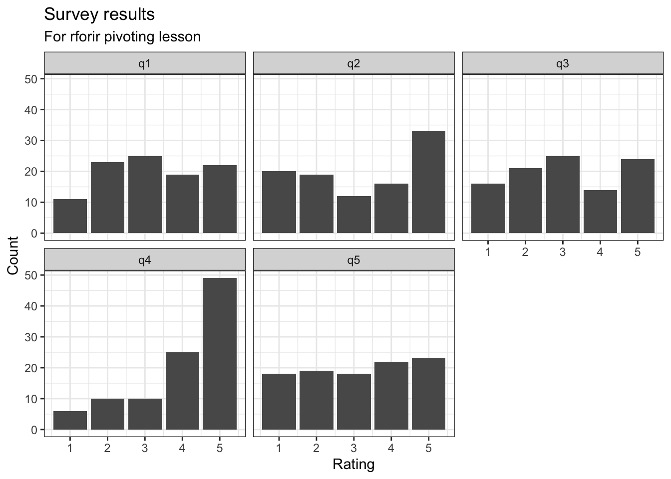
7.1 With a plot
One thing that we can do is plot the results using the functionality of ggplot (part of the tidyverse).
7.2 With a table
Or we could summarize in a table (by using the pivot_wider() function that we explored above):
7.3 With statistics
Or just numerical summaries using group_by() and summarize():
An advantage of the code above is that it will work for any survey with discrete responses, no matter how long it is or what the columns are called. This greatly facilitates automation of reporting.