students <-
  tibble(id = 1:5,
         given_name = c("Al", "Bob", "Charles", "Dave", "Ed"),
         family_name = c("Adams", "Barker", "Cook", "Davidson", "Edwards"))
jobs <-
  tibble(id = 1:5,
         title = c("Analyst", "Baker", "Cook", "Dog Catcher", "Evangelist"))
clubs <-
  tibble(id = 1:5,
         title = c("Archery", "Badminton", "Chess", "Dahlias", "Eating"))
employment <-
  tibble(student = c(1, 1, 2, 2),
         job = c(1, 3, 3, 4))
membership <-
  tibble(student = c(2, 2, 3, 5),
club = c(1, 4, 4, 5))Joins
Working with data from multiple data frames
1 Overview & introduction
1.1 What you’ve learned about
R&RStudio- packages:
tidyverse,knitr,kableExtra - data types
select(),filter(),|>,mutate()
- factors (advanced)
pivot_wider(),pivot_longer()group_by(),summarize()- functions
We have a good start on learning the basics of R/tidyverse and those functions that allow us to pivot data and to calculate summary statistics.
1.2 Today
- Joins: lecture & demo
left_join(): in-depth- Reference for other joins
- IPEDS data
- Huge demo
- Large
Rfile (with lots of comments) - Uses lots of the tools we have learned so far
Last week, you learned about pivoting, which is a new kind of operation for most of you. Today, we’re going to be focusing on joins, another new kind of operation for many of you. It is the one, single thing that enables all of this work in R both to be possible and to be challenging mentally.
2 Joins: Bringing data together
Today, we’re going to work with joins. I have used that term a few times without really describing what it is. Let me give it a try:
Joins refer to the action of linking two or more tables together in a way that facilitates analysis. The separation of data into separate tables (in the first place) enables a more logical and consistent structuring of data that is, in turn, easier both to access and to maintain.
2.1 Our data
In this collection of data, we have 5 students, 5 jobs, and 5 clubs. The employment data frame shows the two students who each have two jobs. The `membership data frame shows the three students who are members of clubs (one is a member of two of them).
A feature of this organization of data is that every separate data frame is about one thing, and one thing only.
2.2 Concept: Keys
2.2.1 Primary Keys
- Definition: a column (or set of columns) whose value can be used to identify one-and-only-one row in that data frame.
- Examples:
student.id,club.id,membership.[student, club]
2.2.2 Foreign Keys
- Definition: a column (or set of columns) whose value can be used to identify one-and-only-one row in another data frame. It must be the primary key in that other data frame.
- Examples:
membership.student,employment.job
The primary keys are as follows. Satisfy yourself that each primary key uniquely identifies one-and-only-one row in its data frame.
[students.id][jobs.id][clubs.id]employment.[student, job]membership.[student, club]
The foreign keys are as follows:
employment.studenttostudents.idemployment.jobtojobs.idmembership.studenttostudents.idmembership.clubtoclubs.id
Each single foreign key value refers to one and only one primary key value. However, sometimes one particular primary key value can refer to many different rows where it is embedded as a foreign key.
What if you wanted to add some new pieces of data to this set of data. Where would you put the following columns:
- Date that a club was founded
- Date that a student joined a club
- Date that a student began working at a job
- Possible pay range for a particular job
The answers to these questions can be determined by thinking about what specific primary key would determine the value of each of the above.
Here are my answers:
- Date that a club was founded: Put
founding_dateintoclubs. Each club can have one and only one founding date. - Date that a student joined a club: Put
join_dateintomembership. Each student can join a specific club just one time. - Date that a student began working at a job: Put
start_dateintoemployment. Each student can start a specific job on just one date. - Possible pay range for a particular job: Put
min_pay_rateandmax_pay_rateintojobs. Each job can have one and only one pay range, but that pay range is defined by two values (a minimum and a maximum). Each column should contain one and only one value.
2.3 Entity-Relationship (ER) diagram
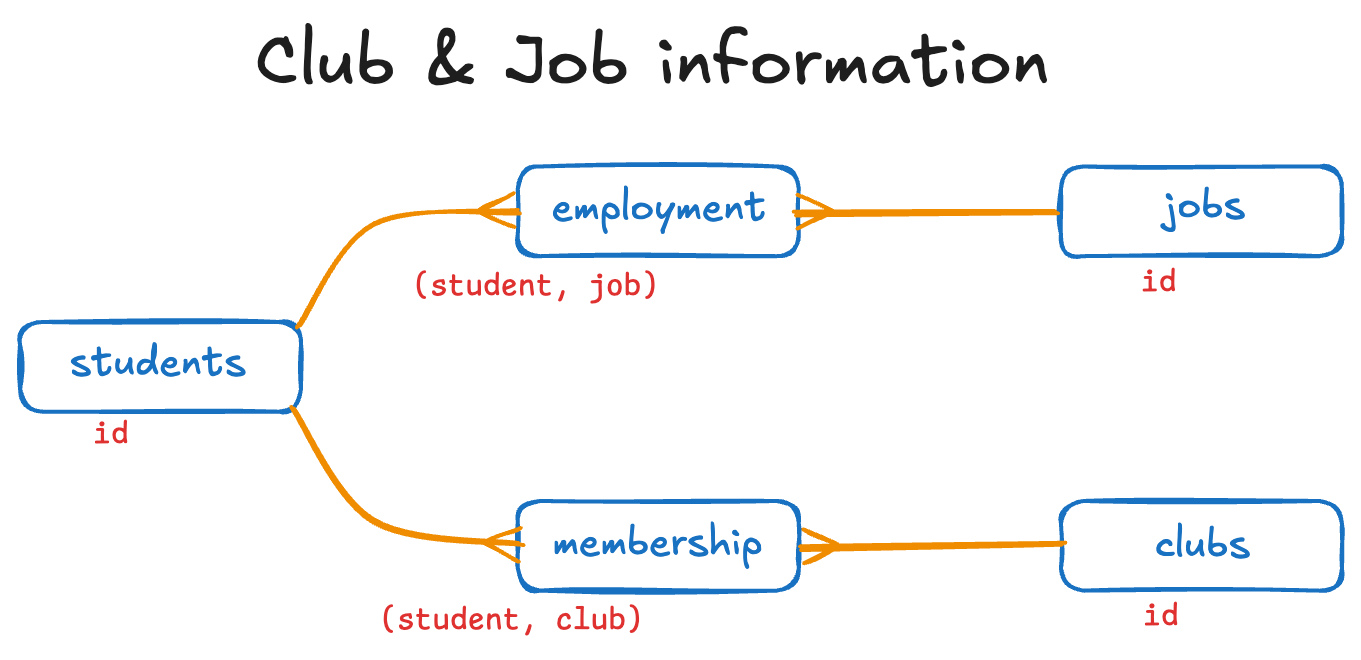
The entities are the boxes. The relationships are the lines.
You read the relationship with the following structure, starting at the single (line) end and moving to the multiple (fork) end:
For every LINE, there can be many FORK. For any single FORK, there can be at most one LINE.
Thus, we have the following represented in this diagram:
- For every student, there can be many employments.
- For every employment, there is one and only one job.
- For every job, there can be many employments.
- For every employment, there is one and only one job.
- For every student, there can be many memberships.
- For every membership, there can be one and only one club.
- For every club, there can be many memberships.
- For every membership, there can be one and only one student.
The red text below each entity is the primary key. You should find a foreign key in the FORK END that refers to the primary key at the LINE END.
3 Joins
3.1 Joins and Primary and Foreign Keys
- Joins are the way that the
R/tidyversebrings together (joins!) data from multiple data frames. - Primary and foreign keys within the data are what enables this to work.
- This concept is applicable in all databases (since the 1970s).
- These are called relational databases.
- This is also applicable to all analytic software (e.g.,
R,Tableau, etc.). - And this is so much faster than
vlookup()from Excel.- It’s built-in to databases rather than being an add-on.
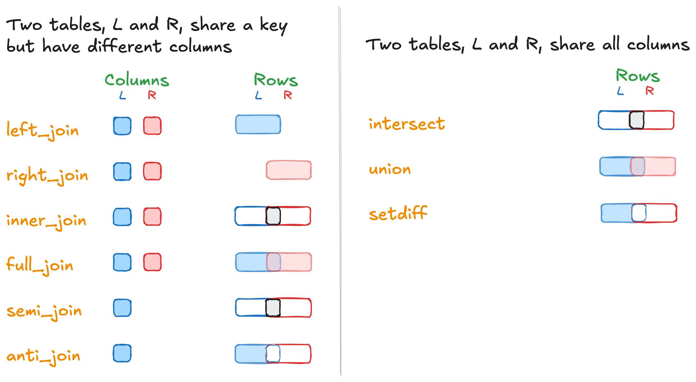
3.2 Types of joins
R/tidyversehas six kinds of joins.- We will look at just one of them
- …but this document can serve as a reference to all of them.
3.3 Options for joining tables together
3.4 left_join(): example 1
The question: List all students with the club names, if any, that they belong to.
left_join: added one column (club)
> rows only in students 2
> rows only in membership (0)
> matched rows 4 (includes duplicates)
> ===
> rows total 6
left_join: added one column (title)
> rows only in left_join(students, mem.. 2
> rows only in clubs (2)
> matched rows 4
> ===
> rows total 6# A tibble: 6 × 5
id given_name family_name club title
<dbl> <chr> <chr> <dbl> <chr>
1 1 Al Adams NA <NA>
2 2 Bob Barker 1 Archery
3 2 Bob Barker 4 Dahlias
4 3 Charles Cook 4 Dahlias
5 4 Dave Davidson NA <NA>
6 5 Ed Edwards 5 Eating We’re traversing in the ER diagram starting at student and going down a fork and then up a line (from students to membership to clubs). Note that the columns going across are in order by when they were encountered. club is picked up from membership (but not student since it is replicated by id which is already there) and then title is picked up from clubs (but not id since it is replicated by club which is already there).
When specifying the join_by() columns, we ensure that we are including the whole and correct primary and foreign keys.
3.5 left_join(): example 2
The question: List all students with the club names, if any, that they belong to.
students |>
  left_join(membership, join_by(id == student)) |>
left_join(clubs, join_by(club == id)) |>
mutate(full_name = str_c(given_name, " ", family_name)) |>
select(full_name, title)left_join: added one column (club)
> rows only in students 2
> rows only in membership (0)
> matched rows 4 (includes duplicates)
> ===
> rows total 6
left_join: added one column (title)
> rows only in left_join(students, mem.. 2
> rows only in clubs (2)
> matched rows 4
> ===
> rows total 6
mutate: new variable 'full_name' (character) with 5 unique values and 0% NA
select: dropped 4 variables (id, given_name, family_name, club)# A tibble: 6 × 2
full_name title
<chr> <chr>
1 Al Adams <NA>
2 Bob Barker Archery
3 Bob Barker Dahlias
4 Charles Cook Dahlias
5 Dave Davidson <NA>
6 Ed Edwards Eating The question here is the same, so this query starts out the same as the previous query. The difference is that this time we have chosen to list just the student’s full name and the title of the club.
The str_c() function concatenates the three text strings and puts the result in the new full_name column. The select() statement directs the R/tidyverse to display just two columns.
3.6 left_join(): the workhorse
- Description: All info from left plus possible matches with right
- Rows included: all from left
- Columns included: all from left and all from right (with NAs when no match is found)
- You will probably use this 90% of the time
- Template
3.7 Aside: join_by()
You have three options for specifying how the two data frames are to be joined:
join_by(LEFTKEY == RIGHTKEY): Is always appropriate.join_by(KEYNAME): When theLEFTKEYandRIGHTKEYare named the same.- nothing at all: When the
LEFTKEYandRIGHTKEYare named the same and are the only two columns in the two data frames that have the same names.- This one makes me nervous because it can fail without giving an error.
3.8 right_join()
- Description: All info from right plus possible matches with left
- Rows included: all from right
- Columns included: all from right and all from left (with NAs when no match is found)
- Template
3.9 right_join(): example (part a)
The question: List the student names and job titles for only students with jobs.
right_join: added one column (job)
            > rows only in students   (3)
            > rows only in employment  0
            > matched rows             4
            >                         ===
> rows total 4| id | given_name | family_name | job |
|---|---|---|---|
| 1 | Al | Adams | 1 |
| 1 | Al | Adams | 3 |
| 2 | Bob | Barker | 3 |
| 2 | Bob | Barker | 4 |
We’re doing this in three stages.
In this first stage, we want to complete the first join. We choose a right join so that we have all the information from students but only for those students who have a job (i.e., they are in the employment data frame).
3.10 right_join(): example (part b)
The question: List the student names and job titles for only students with jobs.
students |>
  right_join(employment, join_by(id == student)) |>
  left_join(jobs, join_by(job == id)) |>
  kbl() |> kable_minimal()
right_join: added one column (job)
> rows only in students (3)
> rows only in employment 0
> matched rows 4
> ===
> rows total 4
left_join: added one column (title)
> rows only in right_join(students, em.. 0
> rows only in jobs (2)
> matched rows 4
> ===
> rows total 4| id | given_name | family_name | job | title |
|---|---|---|---|---|
| 1 | Al | Adams | 1 | Analyst |
| 1 | Al | Adams | 3 | Cook |
| 2 | Bob | Barker | 3 | Cook |
| 2 | Bob | Barker | 4 | Dog Catcher |
In this second stage, we complete the second join. We use a left_join() because every row in employment will have an associated row in the jobs data frame (since jobs.job is never empty).
3.11 right_join(): example (part c)
The question: List the student names and job titles for only students with jobs.
students |>
  right_join(employment, join_by(id == student)) |>
  left_join(jobs, join_by(job == id)) |>
  mutate(full_name = str_c(given_name, family_name, sep = " ")) |>
  select("Full name" = full_name, "Job title" = title) |>
  kbl() |> kable_minimal()
right_join: added one column (job)
> rows only in students (3)
> rows only in employment 0
> matched rows 4
> ===
> rows total 4
left_join: added one column (title)
> rows only in right_join(students, em.. 0
> rows only in jobs (2)
> matched rows 4
> ===
> rows total 4
mutate: new variable 'full_name' (character) with 2 unique values and 0% NA
select: renamed 2 variables (Full name, Job title) and dropped 4 variables| Full name | Job title |
|---|---|
| Al Adams | Analyst |
| Al Adams | Cook |
| Bob Barker | Cook |
| Bob Barker | Dog Catcher |
In this third stage, we improve the formatting of the name and the column headers.
3.12 inner_join()
- Description: All info from right and left but only when there is a match
- Rows included: only those rows when there is a match
- Columns included: all from right and all from left
- Template
3.13 inner_join(): example 1
The question: How many students have both a job and membership in a club?
Note the simplified join_by().
inner_join: added one column (club)
            > rows only in employment (2)
            > rows only in membership (2)
            > matched rows             4    (includes duplicates)
            >                         ===
            > rows total               4
select: dropped 2 variables (job, club)
[1] 1Both employment and membership have foreign keys that reference the primary key of students. As such, we can skip including students and simply do a join between these two data frames. Since an inner_join requires that the key be in both tables (and since all columns from both tables would be included), we could have written the query like this:
The select() ensures that just student (the student’s id) remains and then n_distinct() counts the number of distinct values (i.e., students) remain.
3.14 inner_join(): example 2
The question: List the full names, job titles, and clubs, for only those students who have both a job and membership in a club.
employment |>
  inner_join(membership, join_by(student)) |>
  left_join(students, join_by(student == id)) |>
  left_join(jobs, join_by(job == id)) |>
  left_join(clubs, join_by(club == id)) |>
  mutate(full_name = str_c(family_name, ", ", given_name)) |>
  select(full_name, Job = title.x, Club = title.y)
inner_join: added one column (club)
> rows only in employment (2)
> rows only in membership (2)
> matched rows 4 (includes duplicates)
> ===
> rows total 4
left_join: added 2 columns (given_name, family_name)
> rows only in inner_join(employment, .. 0
> rows only in students (4)
> matched rows 4
> ===
> rows total 4
left_join: added one column (title)
> rows only in left_join(inner_join(em.. 0
> rows only in jobs (3)
> matched rows 4
> ===
> rows total 4
left_join: added 2 columns (title.x, title.y)
> rows only in left_join(left_join(inn.. 0
> rows only in clubs (3)
> matched rows 4
> ===
> rows total 4
mutate: new variable 'full_name' (character) with one unique value and 0% NA
select: renamed 2 variables (Job, Club) and dropped 5 variables# A tibble: 4 × 3
full_name Job Club
<chr> <chr> <chr>
1 Barker, Bob Cook Archery
2 Barker, Bob Cook Dahlias
3 Barker, Bob Dog Catcher Archery
4 Barker, Bob Dog Catcher DahliasThis time instead of a count we are looking for information about the students, jobs, and clubs. Let’s explain the four joins:
employment |> inner_join(membership, join_by(student))-
Results in a data frame with
student, job, clubfor all of those students who have both a job and membership in a club. |> left_join(students, join_by(student == id))-
We are joining the result of the previous join with
students. We are ensuring that the existingstudentconnects to the row in thestudentsdata frame for which it matches theidcolumn. The result is a data frame with columnsstudent,job,club,given_name, andfamily_name. But, again, it is only for those students who have both a job and membership in a club. |> left_join(jobs, join_by(job == id))-
We are joining the result of the previous join with
jobs. We are ensuring that the existingjobcolumn matches theid(primary key) column ofjobs. This adds thetitlecolumn fromjobsto the existing set of columns (but without adding any rows). |> left_join(clubs, join_by(club == id))-
We are joining the result of the previous join with
clubs. We are ensuring that the existingclubcolumn matches theid(primary key) column ofclubs. This adds thetitlecolumn fromclubsto the existing set of columns.
Note carefully the following: Since we added a title column in the third join and in the fourth join, and since column names have to be unique, R/tidyverse renames the columns to title.x and title.y. We could have avoided this by using rename() after the third join but we generally just let the R/tidyverse handle it first and then we clean it up later.
After those four joins, we use mutate() to calculate a new full_name column. We then use select() to both choose the columns that we want to display and also rename both the title columns.
3.15 full_join()
- Description: All info from left and right
- Rows included: all from left and right
- Columns included: all from left (with NAs when no match is found) and all from right (with NAs when no match is found)
- Template
3.16 full_join(): example 1 (part a)
The question: List the ids and first and given names for all students who have either a job or club membership.
(students_with_jobs_or_clubs <- membership |>
  full_join(employment, join_by(student)) |>
  select(student))
full_join: added one column (job)
> rows only in membership 2
> rows only in employment 2
> matched rows 4 (includes duplicates)
> ===
> rows total 8
select: dropped 2 variables (club, job)# A tibble: 8 × 1
student
<dbl>
1 2
2 2
3 2
4 2
5 3
6 5
7 1
8 1We are, again, going to approach this example in three stages.
In this first stage, we define a data frame students_with_jobs_or_clubs that contains just the student id (student) for those students who are members of a club or have a job.
3.17 full_join(): example 1 (part b)
The question: List the ids and first and given names for all students who have either a job or club membership.
left_join: added no columns
           > rows only in students                   1
           > rows only in students_with_jobs_or_c.. (0)
           > matched rows                            8    (includes duplicates)
           >                                        ===
           > rows total                              9
# A tibble: 9 × 3
id given_name family_name
<dbl> <chr> <chr>
1 1 Al Adams
2 1 Al Adams
3 2 Bob Barker
4 2 Bob Barker
5 2 Bob Barker
6 2 Bob Barker
7 3 Charles Cook
8 4 Dave Davidson
9 5 Ed Edwards With this query we can get all the information from the students data frame by performing this left_join() from students to the data frame we just created.
3.18 full_join(): example 1 (part c)
The question: List the ids and first and given names for all students who have either a job or club membership.
students |>
  left_join(membership |>
              full_join(employment, join_by(student)) |>
              select(student),
            join_by(id == student))
full_join: added one column (job)
> rows only in membership 2
> rows only in employment 2
> matched rows 4 (includes duplicates)
> ===
> rows total 8
select: dropped 2 variables (club, job)
left_join: added no columns
> rows only in students 1
> rows only in select(full_join(member.. (0)
> matched rows 8 (includes duplicates)
> ===
> rows total 9# A tibble: 9 × 3
id given_name family_name
<dbl> <chr> <chr>
1 1 Al Adams
2 1 Al Adams
3 2 Bob Barker
4 2 Bob Barker
5 2 Bob Barker
6 2 Bob Barker
7 3 Charles Cook
8 4 Dave Davidson
9 5 Ed Edwards The trick shown here is a little mind-blowing. What’s going on?
- The first argument of
left_joinmust be a data frame. - The query
membership |> full_join(...) |> select(...)is the same query that we used in part a to definestudents_with_jobs_or_clubs. - Here we simply substituted the query itself for the name of the data frame that the query was used to create. (Compare them yourselves!)
The R/tidyverse is flexible enough that it can substitute a query for the name of a data table. Who knew?!?
We don’t expect you to use this approach much, but we wanted you to know about it so that you don’t get overly alarmed if you come across it elsewhere.
3.19 full_join(): example 2
The question: List the IDs and first and given names for all students who have either a job or club membership.
students |>
  right_join(employment |>
               full_join(membership, join_by(student)),
             join_by(id == student)) |>
  distinct(id, given_name, family_name)
full_join: added one column (club)
> rows only in employment 2
> rows only in membership 2
> matched rows 4 (includes duplicates)
> ===
> rows total 8
right_join: added 2 columns (job, club)
> rows only in students (1)
> rows only in full_join(employment, m.. 0
> matched rows 8
> ===
> rows total 8
distinct: removed 4 rows (50%), 4 rows remaining# A tibble: 4 × 3
id given_name family_name
<dbl> <chr> <chr>
1 1 Al Adams
2 2 Bob Barker
3 3 Charles Cook
4 5 Ed Edwards Except for the last line, this query is the same as the last one. The distinct() command enables us to get rid of all of the duplicate students.
3.20 anti_join()
- Description: All info from left
- Rows included: all from left that are not in right
- Columns included: all from left
- Template
3.21 anti_join(): example 1
The question: List the ids and names of all students who do not have a job.
anti_join: added no columns
           > rows only in students    3
           > rows only in employment (0)
           > matched rows            (2)
           >                         ===
           > rows total               3
# A tibble: 3 × 3
id given_name family_name
<int> <chr> <chr>
1 3 Charles Cook
2 4 Dave Davidson
3 5 Ed Edwards The anti_join() is the perfect command for this question. It looks at all the id values in students and chooses only those that are not in the student column of employment. That is, it displays those students who do not have a job! Easy peasy.
3.22 anti_join(): example 2
The question: List the ids and names of all students and their clubs who are in a club but do not have a job.
membership |>
    anti_join(employment, join_by(student)) |>
    left_join(students, join_by(student == id)) |>
    left_join(clubs, join_by(club == id)) |>
    mutate(full_name = str_c(given_name, " ", family_name)) |>
    select(StID = student,
           `Full Name` = full_name,
           Club = title) |>
    kbl() |> kable_minimal()
anti_join: added no columns
> rows only in membership 2
> rows only in employment (2)
> matched rows (2)
> ===
> rows total 2
left_join: added 2 columns (given_name, family_name)
> rows only in anti_join(membership, e.. 0
> rows only in students (3)
> matched rows 2
> ===
> rows total 2
left_join: added one column (title)
> rows only in left_join(anti_join(mem.. 0
> rows only in clubs (3)
> matched rows 2
> ===
> rows total 2
mutate: new variable 'full_name' (character) with 2 unique values and 0% NA
select: renamed 3 variables (StID, Full Name, Club) and dropped 3 variables| StID | Full Name | Club |
|---|---|---|
| 3 | Charles Cook | Dahlias |
| 5 | Ed Edwards | Eating |
By executing an anti_join() from membership to employment, we are choosing those students who are in a club but do not have a job (which is what we wanted).
Now, since we want all the student information, we need to left_join to students. Since every student in membership is in students, we do not have to worry about inserting any NA values.
The third join, a left_join() with clubs, gets us the name of the club (the title column).
We then use mutate() to calculate the full_name column, select() to give three columns more informative names, and then the kable commands to format the table display.
3.23 semi_join()
- Description: all info from left but only for those that are also in right
- Rows included: all from left that match in right
- Columns included: only those from left
- Template
3.24 semi_join(): example 1
The question: List those students who have jobs.
semi_join: added no columns
> rows only in students (3)
> rows only in employment (0)
> matched rows 2
> ===
> rows total 2# A tibble: 2 × 3
id given_name family_name
<int> <chr> <chr>
1 1 Al Adams
2 2 Bob Barker This semi_join() statement selects all of the columns from students but only those rows for which students.id is in the student column of employment. That is, it lists all student information for those students who have jobs.
3.25 semi_join(): example 2
The question: List students who have both jobs and membership in clubs.
students |>
semi_join(employment, join_by(id == student)) |>
semi_join(membership, join_by(id == student))semi_join: added no columns
> rows only in students (3)
> rows only in employment (0)
> matched rows 2
> ===
> rows total 2
semi_join: added no columns
> rows only in semi_join(students, emp.. (1)
> rows only in membership (2)
> matched rows 1
> ===
> rows total 1# A tibble: 1 × 3
id given_name family_name
<int> <chr> <chr>
1 2 Bob Barker This query starts the same as the previous one. Let’s explain what happens:
students |> semi_join(employment,...)-
Again, this has selected all student information for those students who have jobs. The result is a data frame with the same columns as are in
studentsbut fewer rows (since not all students have jobs). |> semi_join(membership,...)- Now, taking the input from the previous join, this join selects only those rows for students that are members of a club.
After going through both joins, the result is the set of students who have both a job and membership in a club.
4 Set operators
4.1 R’s three set operators
R has three basic set operators that work with two data frames with the exact same columns:
intersect(LEFT_DF, RIGHT_DF): the rows are in bothunion(LEFT_DF, RIGHT_DF): the rows are in either one (but only one is included)setdiff(LEFT_DF, RIGHT_DF): the row is in the left but not the right
4.2 intersect(): example
Question: List all the students who both are a member of a club and have a job.
intersect(
students |> semi_join(membership, join_by(id == student)),
students |> semi_join(employment, join_by(id == student))
)semi_join: added no columns
> rows only in students (2)
> rows only in membership (0)
> matched rows 3
> ===
> rows total 3
semi_join: added no columns
           > rows only in students   (3)
           > rows only in employment (0)
           > matched rows             2
           >                         ===
           > rows total               2
# A tibble: 1 × 3
id given_name family_name
<int> <chr> <chr>
1 2 Bob Barker The intersect() command has two data frame arguments:
- The first one is the set of students who are club members.
- The second one is a set of students who have jobs.
The result of this is a set of students who are in both data frames; that is, these students have both a job and a club membership.
By the way, a set by definition, cannot have duplicate items in it.
4.3 union(): example
Question: List all the students who are either a member of a club or have a job.
union(
  students |> semi_join(membership, join_by(id == student)),
  students |> semi_join(employment, join_by(id == student))
) |>
  arrange(id)
semi_join: added no columns
> rows only in students (2)
> rows only in membership (0)
> matched rows 3
> ===
> rows total 3
semi_join: added no columns
> rows only in students (3)
> rows only in employment (0)
> matched rows 2
> ===
> rows total 2# A tibble: 4 × 3
id given_name family_name
<int> <chr> <chr>
1 1 Al Adams
2 2 Bob Barker
3 3 Charles Cook
4 5 Ed Edwards The union() command also has two data frame arguments; in this case, the same as the previous example. The result of this is a set of students who are in either one set or the other. That is, these students have either a job or a club membership.
The arrange() command ensures that the results are sorted by id.
4.4 setdiff(): example
Question: List all the students who are in a club but do not have a job.
setdiff(
  students |> semi_join(membership, join_by(id == student)),
  students |> semi_join(employment, join_by(id == student))
)
semi_join: added no columns
> rows only in students (2)
> rows only in membership (0)
> matched rows 3
> ===
> rows total 3
semi_join: added no columns
> rows only in students (3)
> rows only in employment (0)
> matched rows 2
> ===
> rows total 2# A tibble: 2 × 3
id given_name family_name
<int> <chr> <chr>
1 3 Charles Cook
2 5 Ed Edwards The setdiff() command is used to perform a subtraction. It subtracts the second data frame from the first. The arguments to this command are the same as the previous two examples. The result is a set of students who have a club membership but not a job.
5 In-class demo & then Homework
5.1 The data model
6 Coming up
6.1 Dates
- Joins
- Monday, Feb 24: Week 3
- Wednesday, Feb 26: Problem session
- Bringing it all together
- Monday, March 3
- Wednesday, March 5: Problem session
- Week for you to work on your project
- Project presentations
- Monday, March 17
6.2 Work on the following
- Refer to the week 3 slide page and read through it.
- Complete the Joins lesson.
- Read through the file
create_ipeds_data_frame.R - Do the homework (at end of previous file).
- You will be sending us the results of your work!
- FYI, next week we will work with joins quite extensively both in class and in your homework.