   record_id        student_id       section_id          subject
 Min.   :   1.0   Min.   :  1.00   Min.   : 1.00   Biology   :232
 1st Qu.: 250.8   1st Qu.: 26.00   1st Qu.:13.00   Chemistry :247
 Median : 500.5   Median : 51.00   Median :25.50   Economics :269
 Mean   : 500.5   Mean   : 51.27   Mean   :25.53   Psychology:252
 3rd Qu.: 750.2   3rd Qu.: 77.00   3rd Qu.:38.00
 Max.   :1000.0   Max.   :100.00   Max.   :50.00
  grade_points   grade_letter
 Min.   :0.800   F:  1
 1st Qu.:3.000   D: 19
 Median :3.500   C:194
 Mean   :3.358   B:733
 3rd Qu.:3.800   A: 53
Max. :4.000 Pivoting, groups, and functions
1 Overview & introduction
1.1 What you’ve learned about
RRStudio- packages
tidyverse
- data types
select()filter()|>mutate()- factors (advanced)
We have a good start on learning the basics of R/tidyverse. The first step in learning this language is to understand each of these operators and concepts individually. The complexity of this approach really comes when you combine them in order to get work done. This gets easier with practice…but it does take practice and time.
1.2 Today
- Summary statistics
group_by()summarize()mean(),median(),max(),min()
- Pivoting:
pivot_wider()&pivot_longer() - Functions
- In-class demo: survey data
- Collaboration (and starting the homework): IPEDS data
Today we are definitely getting to more complex operators. It’s not that they are obtuse; they just have more nuances than what we have previously learned.
What we’re going to do today in class is go through these slides and get an overview of these topics. Then we’re going to go through an in-class demo. We’ll finish by getting familiar with the data and files that you’re going to work with on your homework.
2 Calculating summary statistics
The first topic that we’re going to review relates to calculating summary statistics. We’re going to be working with a grades data frame that we are generating dynamically (i.e., there isn’t a CSV file associated with this example.
2.1 Summary of grades data
Here is the data. We have 1000 rows of data with these six columns:
record_id- the unique identifier for the row
student_id- the unique identifier for the student. One hundred students are represented in this data frame.
section_id- The section number of a course that the student took. Fifty students are represented in this data frame.
subject- The department name that offered the course. Four departments are in this data frame.
grade_points- The grade points the student earned in this class. The possible range is from 0 to 4.0.
grade_letter-
The letter grade the student earned in this class. The possible range is
c(F, D, C, B, A)(from low to high).
2.2 Top of the grades data frame
| record_id | student_id | section_id | subject | grade_points | grade_letter |
|---|---|---|---|---|---|
| 1 | 68 | 26 | Psychology | 3.8 | B |
| 2 | 86 | 42 | Biology | 2.8 | C |
| 3 | 80 | 48 | Biology | 3.8 | B |
| 4 | 37 | 50 | Chemistry | 3.1 | B |
| 5 | 50 | 40 | Chemistry | 3.9 | B |
| 6 | 95 | 41 | Biology | 2.5 | C |
| 7 | 95 | 38 | Economics | 2.9 | C |
| 8 | 14 | 22 | Psychology | 3.4 | B |
| 9 | 18 | 38 | Economics | 2.9 | C |
Here’s a look at the first 9 rows of the data frame. It looks just about how you might expect.
2.3 Three standard ways to summarize data
- Vector-based
summarize()for whole data framesummarize()withgroup_by()for parts of data frame
We’re going to go through three standard ways that R provides for calculating summary data. Much more detail is provided in the lessons that you will complete this week. I just want to introduce each of the approaches.
2.4 Vector-based statistics
The first way is to use a function and apply it to a vector of numerical data.
2.5 summarize() for whole data frame
grades |>
  summarize(min = min(grade_points),
            avg = mean(grade_points),
            max = max(grade_points)) |>
  kable(digits = 2)
summarize: now one row and 3 columns, ungrouped| min | avg | max |
|---|---|---|
| 0.8 | 3.36 | 4 |
This second approach uses the R/tidyverse. Now we can calculate on the whole data frame multiple statistics at the same time.
Note the kable() operator that cleans up the presentation of data frames. You have to load the knitr package.
2.6 summarize() with group_by()
grades |>
  group_by(Subject = subject) |>
  summarize(Min = min(grade_points),
            Avg = mean(grade_points),
            Max = max(grade_points)) |>
  kable(digits = 2)
group_by: one grouping variable (Subject)
summarize: now 4 rows and 4 columns, ungrouped| Subject | Min | Avg | Max |
|---|---|---|---|
| Biology | 1.5 | 3.34 | 4 |
| Chemistry | 1.2 | 3.36 | 4 |
| Economics | 1.4 | 3.40 | 4 |
| Psychology | 0.8 | 3.33 | 4 |
This naturally leads one to think about…“but what are the statistics for each subject?”
This is where the group_by() operator comes in. It needs to have one or more column names in it.
3 Pivoting
Okay, that was it for summary statistics. You’ll use those operators a lot.
Now we’re going to talk about pivoting data. This is new concept for those of you who have not worked with analytical software before (such as R or Tableau).
I’m going to clarify what is meant by these terms and then show you, as clearly as I could determine, how to work with the functions that the R/tidyverse supplies to convert between the two formats.
3.1 Comparing the data structures
3.1.1 Wide
- Typical of spreadsheet data
- Lots of columns containing comparable data
Rhas functions to convert from wide to long- Can be useful when trying to visualize tables of data
3.1.2 Long
- Typical of data for analytical software
R,Tableau, databases
- One column containing all the comparable data
Rhas functions to convert from long to wide- Is beneficial for analytic functions
3.2 Wide (spreadsheet) data
Image of the contents of pivot_ex.xlsx:
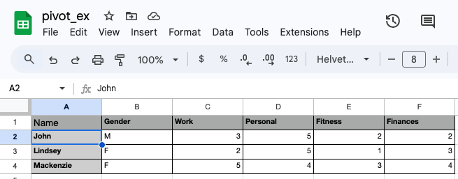
This is the example that we are going to go through. This is all the data from an Excel spreadsheet — 3 rows of 6 columns. This shows data related to how three people rate their lives in different dimensions. It has one identifier column (Name) and one descriptor column (Gender) along with the four data columns.
3.3 Reading in the Excel file
# A tibble: 3 × 6
  Name      Gender  Work Personal Fitness Finances
  <chr>     <chr>  <dbl>    <dbl>   <dbl>    <dbl>
1 John      M          3        5       2        2
2 Lindsey   F          2        5       1        3
3 Mackenzie F 5 4 3 4View(score_df):
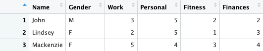
I’ve used the read_xlsx() operator (from the readxl package) to read the Excel spreadsheet into R.
This is our example of wide data — it has four columns that contain data that you might want to compare. It also has one column that you might use to group or filter the data.
3.4 Convert from wide to long
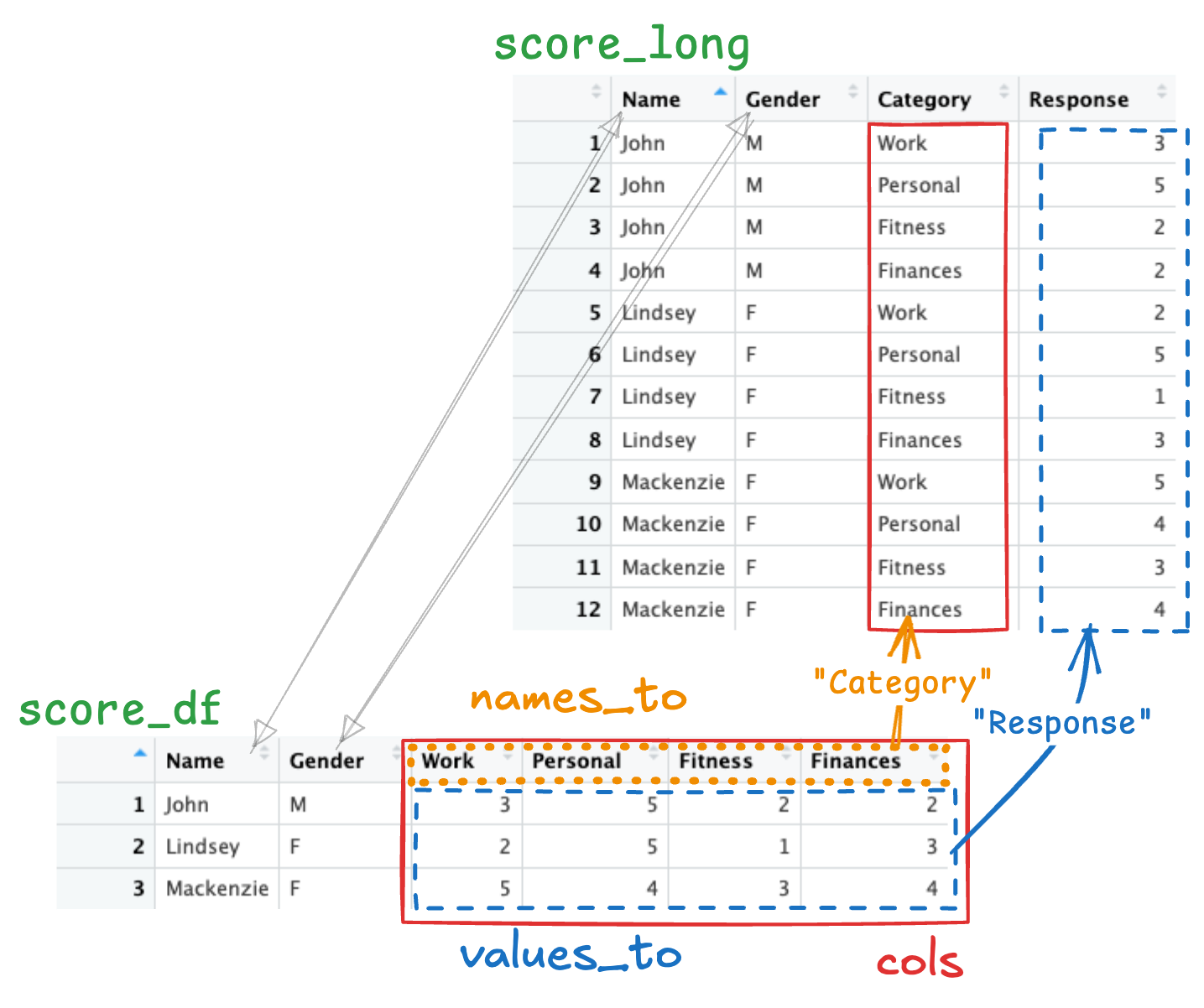
The function pivot_longer() converts data frames from wide to long.
Make sure you understand the transformation that has taken place from score_df (wide) to score_long (long).
You need to make three decisions in order to use this function:
- What columns are going to be pivoted wider?
- In the new long data frame, what will be the name of the column containing the data names?
- In the new long data frame, what will be the name of the column containing the data values?
3.5 Convert from long to wide
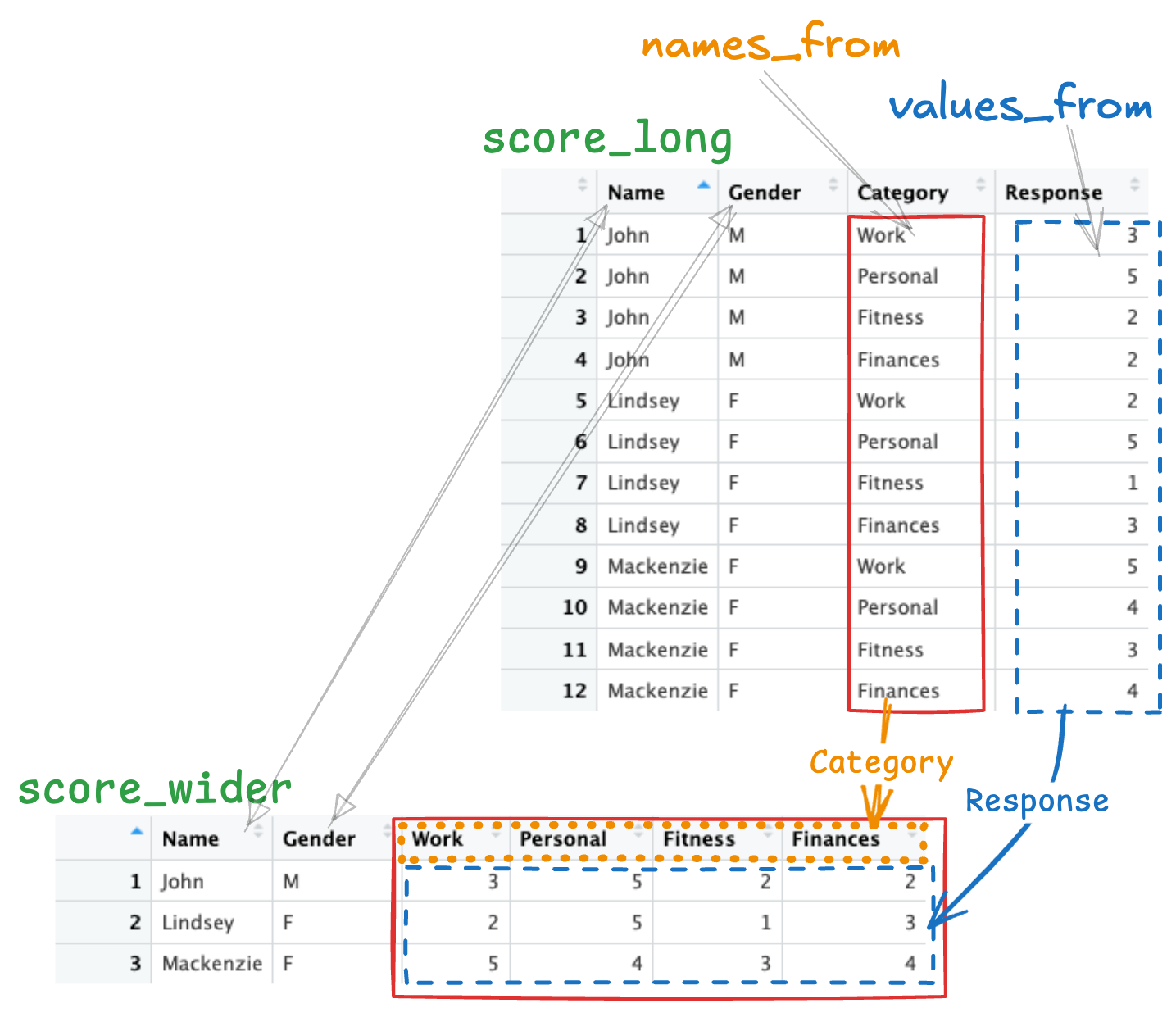
The function pivot_wider() converts data frames from long to wide.
This is simply the reflection of the previous transformation.
You need to make two decisions:
- Which column contains the names of the data values?
- Which column contains the data values?
4 Functions
4.1 R functions
- You’ve already dealt with 10+ functions (
min(),max(), etc.) R(including packages) has 10s of 1000s of functions- Packages are a good way of organizing them
- But the need still arises to define your own
You won’t have to define your own function very frequently at this point. But we wanted you to at least see how it’s done.
4.2 How to define a function
4.2.1 Template
4.2.2 Example 1
A function’s parameters might also be called its arguments.
4.3 Sample function: cell_fmt(n,total)
5 In-class demo & then Homework
6 Coming up
6.1 Dates
- Wednesday, Feb 12: Problem session
- Monday, Feb 17: No class
- Wednesday, Feb 19: No class
- Monday, Feb 24: Week 3 on Joins
- Wednesday, Feb 26: Problem session
We meet again in a couple of days; we thought last week’s session was quite useful. It was free-flowing and, as we wanted, we got a wide variety of questions and addressed all kinds of issues. We look forward to seeing you again.
We’re off next week (in terms of class meetings) but this week’s lessons and homework are relatively extensive so you should take advantage of the extra time before our next class.
6.2 Work on the following
- Lessons: Go through these first!
- Groups, Pivoting, Character variables, Functions
- Homework
- Do this in the Web page.
- After you complete it, wait a while and go through it again within
RStudio. Try to use the hints in the Web page as little as possible.
- Advanced Lessons (if you feel comfortable with the above Lessons)
- Ungroup
- Finding proportions using logical expressions
- Continue thinking about your personal project.
- Slides will be available beginning tomorrow morning.