Week 4 Homework

Bringing it all together on the university data

1 Using `quarto-live` documents

Within this document are blocks of R code.

Edit the code that is shown in the box. Click on the Run Code button.
Make further edits and re-run that code. You can do this as often as you’d like.
Click the Start Over button to bring back the original code if you’d like.

2 Instructions for this homework

This is a long homework, and you shouldn’t think that you can do it all at once, or even before the class is over. It is meant to be something that you can use to remind yourself about all that we learned in this class. So come back to it periodically and try to answer a question that you haven’t attempted before or that it’s been a while since you’ve done it.
You should definitely try this for the first time within this Web page so that you can access the hints.
However, you should also definitely do this eventually within RStudio so that you can see how the whole “put the output in the workbook” process works.

3 Preliminaries

3.1 Setup

We have loaded both the tidyverse and tidylog packages in the background. If you are working in RStudio, then run the following code at the Console:

library(tidyverse)
library(openxlsx2)
library(kableExtra)

3.2 Load the data

We are now going to load the raw data from the CSV files. If you are working in RStudio, then execute the following code at the Console:

source("source/read_in_university_data.R")

If you are working in this web page, then read in the data and display it by running the following code. Note that this skips the validity checking that happens in the source file above; however, this is a lot of calculations and takes time over this Web connection, so we’re trying to minimize this for you.

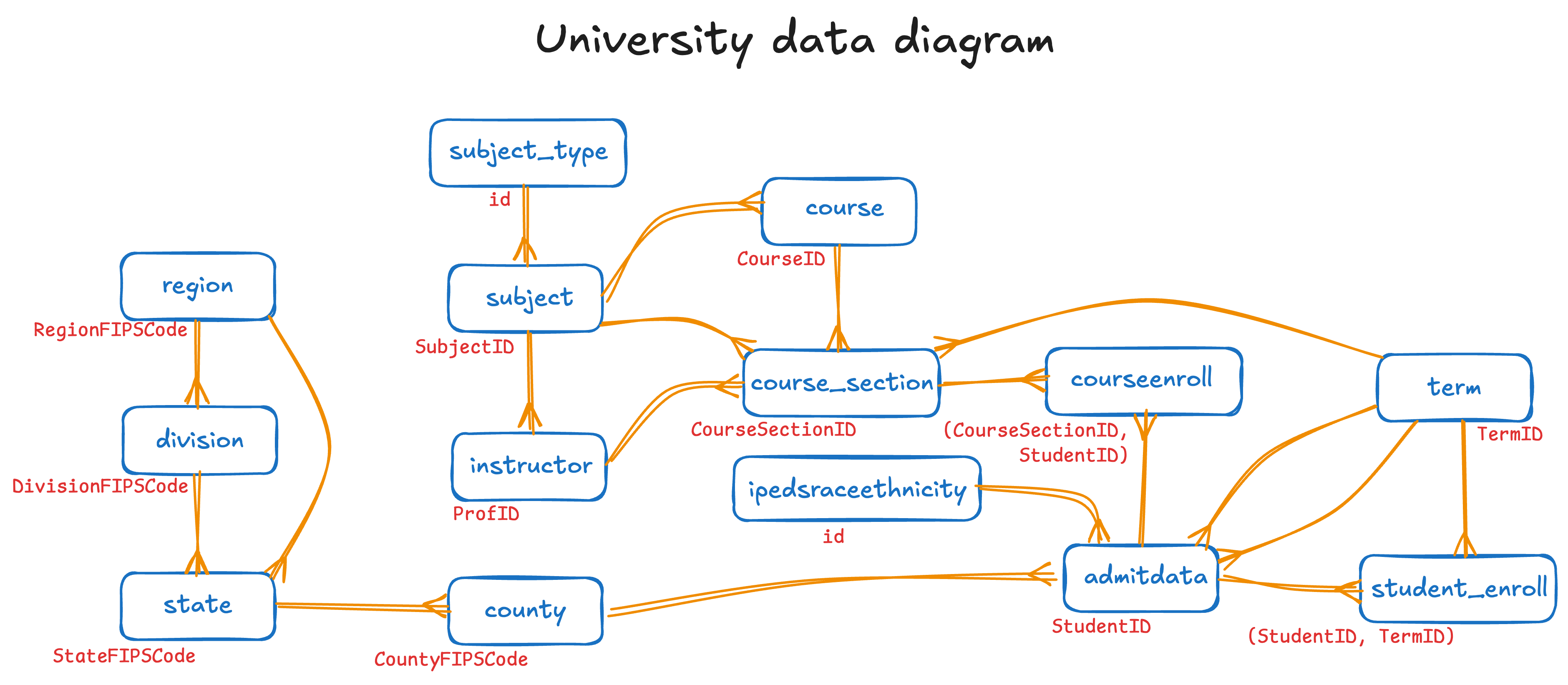
3.3 ER diagram

This is the entity-relationship (ER) diagram for this data set. Let me know if we have missed a relationship or if we could otherwise make this diagram more useful.

Figure 1: ER diagram for the university data set.

We’ll provide this code chunk box that you can use to explore the data as you would like (without having to re-load the data as you would in the above box). We’ll start you out with this code that lists all of the data frames in your global environment.

Tip

What to do if all goes wrong?

If you do something on this page and somehow mess up some data frame, then just run the above code block again. It will reload the data. You can then go back to where you were working.

4 Process that you should follow

For each question in this homework (as for each query you ever construct), you should follow this general process (though we must emphasize that this will be iterative, and you will continually cycle back through this process as you refine your query):

Determine what information you want to display. This will generally rely on your knowleedge of the specific columns in the available data sets. We’ll refer to this as your target data.
Find the data frames that hold that information.
If you have found more than one data frame:
1. Find all the data sets in the ER diagram
2. Determine the path through the ER diagram that you will take to connect all the appropriate data sets
3. Find your base data frame that will serve as the left-most data frame
4. Join the tables together
Filter to include the rows you need
Select the columns you need and rename them if desired
Add groups and calculations (or sort if no groups are needed)
At this point, and only at this point, build the for loops that you need to put the results in different reports or worksheets

In our hints, we will generally proceed in that order — target, data frames, joins, filters, selects, groups, loops.

5 Questions

We have included a link to the ER diagram (Figure 1) at the end of each question because we know how much you will need to refer back to it. (You might also consider printing it out.)

Before you start working on the questions, you need to execute the following. Similarly, if you are working in a script in RStudio, then you should insert this code after you have read in all of the data from the CSV files.

Since you will, almost assuredly, work on these questions over a period of time, even if you work in this Web page (as opposed to RStudio), we encourage you to build up a working R script to capture your answers to each question (and the preliminary setup and reading in of the data). That way, when you are done, you can execute the whole script and enjoy the satisfaction of completing a significant project — and running it again and again with zero additional effort!

Question 1: List instructors

Display the Subject type & name, and Instructor name. List the subjects alphabetically by type, and the instructors alphabetically within subject. (Figure 1)

As a reminder, this is the order to proceed: target, data frames, joins, filters, selects, groups, loops. We’ll get you started.

Targets: For now, we’ll start with Subject Type, Subject Name, and Instructor Name.
Data frames: It looks like, from scanning the ER diagram and the output of the query just below it that lists the column information, we need the data frames instructor, subject, and subject_type.
Joins: This, and the remaining, we leave for you.

We’ll start you off by listing the column names for these three data frames. Until you finish this entire question, we recommend that you leave these three short queries in the code box while you add your answer below it.

So, your first step (and the topic of your first hint) will be to join these data frames together. You, of course, must determine the left-most data frame before you can construct this portion of the query.

Question 2: List courses

Display courses by subject by type. Include information about whether or not they are general ed or major courses. (Figure 1)

Question 3: List courses by subject

Output into a workbook a list of courses (with their credits, audience, and maximum enrollment) by subject. Put each course listing on a separate worksheet. (Figure 1)

Question 4: List counties

Display the Region name, Division name, State name, and County name and the relative size of the county’s labor force (that is, the percentage of its state’s labor force), in descending order of its relative percentage size. This will show which counties in the US make up the largest portion of its state’s labor force. (Figure 1)

Next up: The first thing to do, as always, is determine the targets. For this query, this step is a bit more challenging. Think carefully.

Question 5: Number of students by section

For each section of each course in Fall 2018, calculate the number of students taking that section. Sort by class size within subject. Also show the professor’s name who teaches each section.(Figure 1)

First up: What targets do we have?

Question 6: List courses in a subject by popularity

Output into a workbook, a count of students by course (not course section) in each subject for Spring 2021. Sort in descending order by count within the subject. Create a separate worksheet for each subject. (Figure 1)

Next up: What targets do you have for this query?

Question 7: List low enrolled courses at the university

Output into a workbook, a count of students by course (not course section) for the whole university in Spring 2021. Sort in ascending order by count within the university. List just the courses with counts < 40. (Figure 1)

Question 8: Graduated students per major over the years

What is the number of graduated students per declared major per admitted school year for all years in the data? (Figure 1)

A useful fact to know is that any student who has not graduated has a 0 in the GraduationTerm column of admit_data. If the student has graduated, then that column contains the term ID.

Solution

We want to pivot this long data to wide data and put the admitted school years across the top with table values coming from our previously calculated Num column. Since we also grouped on declared major at the same time, these will be the values down the left side of the table.

Just as a reminder, if you wanted to put these results in a worksheet, then you should add the following lines to the above.

#' Save for later output into an Excel Workbook
wb <- add_ws(wb,
             "GraduatesPerMajorPerAdmitYear",
             "Graduates per major per admit year")
wb <- add_data(wb, graduatesPerMajorPerAdmitYear)
wb <- set_ws_formatting(wb, graduatesPerMajorPerAdmitYear)

Question 9: Average grades per department over the years

For courses offered between Fall 2015-Spring 2022 (inclusive; that is, from term 113 to 126), what is the average grade per department offering it (not per section)? List the results in descending order by the average. (Figure 1)

Question 10: Recent student load by professor

For each department, calculate the number of students taught by each professor per audience type (and in total) over the last six terms. Be sure to print the professor’s name. The results should be sorted descending by total number of students taught. Put the results for each department in a separate worksheet. (Figure 1)

At the very end of your R script in RStudio, add the following line so that it will all be transferred to a workbook.

save_wb(wb, "output/output.xlsx")

Congratulations!

1 Using quarto-live documents

2 Instructions for this homework

3 Preliminaries

3.1 Setup

3.2 Load the data

3.3 ER diagram

4 Process that you should follow

5 Questions

1 Using `quarto-live` documents