Joins – R for the IR Professional

1 Using this document

Within this document are blocks of R code. You can edit and execute this code as a way of practicing your R skills:

Edit the code that is shown in the box. Click on the Run Code button.
Make further edits and re-run that code. You can do this as often as you’d like.
Click the Start Over button to bring back the original code if you’d like.
If the code has a “Test your knowledge” header, then you are given instructions and can get feedback on your attempts.

1.1 Using RStudio

If you’re following along with this exercise in RStudio, then you need to execute the following code in the Console. If you are going through this set of exercises within this document, you don’t have to do so because we are loading this libraries for you.

library(tidyverse)
library(tidylog)
library(kableExtra)

The first line loads the tidyverse package. You could actually load just the packages dplyr and purrr to save on memory, but with today’s computers and the types of things that you’re doing at this point, you don’t need to worry about load speed and/or memory usage just yet.
The second package tells R to give more detailed messages.
The third package allows R/tidyverse to create tables with better formatting.

2 Set up: Create small data frames

A data frame is like a table in a database or a spreadsheet. It has rows and named columns. Most of the time, we load data from a file or database. But for a simple example, we can create one like this.

Listing 1: R code to create data frames for this lesson.

admit_data <- data.frame(
  student = c(2,3,4,5,6,7,7),
  admit_type = c("Regular", "Early", "Regular", 
                 "Early", "Regular", "Regular", 
                 "Regular"),
  first_gen = c(TRUE, NA, TRUE, FALSE, 
                TRUE, TRUE, NA),
  home_address = c(
    "Dayton, OH", "Columbia, SC", "Cleveland, OH", 
    "New York, NY", "Las Vegas, NV", 
    "Cedar Rapids, IA", NA
    )
)
admit_data <- admit_data |>
  mutate(admit_type = factor(admit_type,
                             levels = c("Regular", "Early"),
                             ordered = FALSE))
personal_data <- data.frame(
  id    = c(1, 2, 3, 4, 5, 6, 7),
  first_name = c("Alice", "Bob", "Charlie", 
                 "David", "Eve", "Stanislav", 
                 "Yvette"),
  last_name  = c("Smith", "Jones", "Kline", 
                 "White", "Zettle", "Bernard-Zza", "Zhang")
)
academic_data <- data.frame(
  student    = c(1, 1, 2, 3, 4, 5, 5, 6),
  class      = c("Freshman", "Sophomore", "Sophomore", 
                 "Junior", "Senior", "Senior", 
                 "Senior", "Sophomore"),
  age        = c(17, 18, 18, 19, 20, 
                 21, 21, 19),
  gpa        = c(3.51, 3.48, 3.20, 3.83, 3.03, 3.98, 3.93, 2.91),
  major      = c(NA, "English", "History", 
                 "Biology", "History", "English", 
                 "English", "Computer Science")
)
academic_data <- academic_data |>
  mutate(class = factor(class,
                        levels = c("Freshman", "Sophomore", 
                                   "Junior", "Senior"),
                        ordered = TRUE),
         major = factor(major,
                        levels = c("History", "English",
                                   "Computer Science",
                                   "Biology"),
                        ordered = FALSE))

If you are running this in RStudio, then you should copy the code above, paste it into RStudio, and run it. This will create the data frames necessary to run through the following lesson.

3 Main idea

Merging data between multiple sources is a common task in IR work. These can be easily accomplished in R/tidyverse with the left_join() function and its cousins. For more information on all of this, see this page on rforir. Another example of the left_join() in action can be seen here.

In this lesson we will go through much of the data science process (see Figure 1), and you will find that joining tables together is a tool applicable throughout the process. Basically, joins are needed — not just optional — in any step in which you’re working with multiple data frames at the same time.

A quick overview of what what we’ll be doing in this lesson:

We don’t have to import the data as we’re simply generating it (see Listing 1) for this lesson. Normally, you would be using read_csv(), read_tsv(), or some other operator to get data into R.
Tidying data (Section 4): In this section, we go through many of the steps that are needed to ensure that the data is of the quality that we need:
- Section 4.1: Read (or construct) an ER diagram (Figure 2) to help gain an initial understanding of the relationships among different data frames.
- Section 4.2: Find problems with the data.
- Section 4.4: Fix problems with the data.
Understanding data (Section 5): Explore the data through running queries on it.

4 Tidying the data

In real data science work, much more work is typically done on importing and tidying than is done on the rest of the process. Fortunately, the sources from which the data is derived (e.g., student information systems, admissions data systems, and others) is relatively stable. This means that much of the work that you do to import and tidy one set of data ends up being useful on many more sets of data.

Thus, as we go through the following, be heartened rather than discouraged at the amount of work we do! It ends up being beneficial to a multitude of other problems, and you will already have a head-start on those projects even before you start working on them. At the same time, you will have much more confidence in all of your projects because you will have validated the data (to the best of your abilities).

4.1 ER diagram

The usual first step to deepening your understanding of a set of data is to draw an ER diagram (or to refer to one that already exists…if one might ever be that lucky!). See Figure 2.

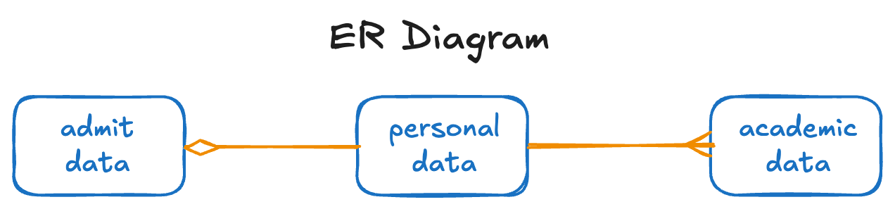
Figure 2: ER diagram for this student data.

Note that you might have come across a similar representation before (especially the orange line on the right) but details about both of the lines might be new to you. Let’s see what this says:

For each row in personal_data, you can have possibly many rows in academic_data. Conversely, for each row in academic_data, you must have one row in personal_data.
For each row in personal_data, you can have possibly one row in admit_data. Conversely, for each row in admit_data, you must have one row in personal_data.

Looking at the actual data frame statements above, we can make the following statements:

It does appear that personal_data contains the data that has to be created first — the person’s id (the primary key) and first and last names. What can be more basic than knowing the name of a person?
The student column in both admit_data and academic_data are foreign keys referencing that primary key in personal_data.
The student column is also the primary key in admit_data.
The primary key for academic_data is [student, class]. In academic_data, each student can have one row for each class of their enrollment.

4.2 Finding problems with the data

Now that we have an initial understanding of the data in the different data frames and how they relate to each other, it is time to begin the process of ensuring that the quality of this data is sufficient for our needs.

4.2.1 Primary key columns

It’s bad news to have a blank primary key column, so we want to check for that. It is also bad news to have duplicate primary key values. Let’s think about why this is the case:

Blank primary key values: The purpose of the primary key is to identify one and only one entity among all of the entities of that type. If the primary key is blank, then we do not know what the rest of the columns in the data frame are about. They are meaningless. Thus, without a value in the primary key column(s), the row can be deleted/ignored.
Duplicate primary key values: Again, the purpose of the primary key is to identify one and only one entity. If a single primary key appears in multiple rows of a data frame, then ambiguity will have reared its ugly head — how do we know which row contains the appropriate information about that particular entity? The answer usually lies in either a quick examination of the data (perhaps one row is comprised of many blank values) or a deeper investigation involving speaking to others who have a deeper insight into how the data was initially created and where it might have originated. In any case, you have to remove the appearance of all duplicates.

The grade data (in academic_data) differs somewhat from the other two data frames. A student may have a row of data for each class of his enrollment (e.g., “Freshman”), resulting in a data frame for which any single student ID might appear in multiple rows, but it should never be the case (in academic_data) that the combination of a student ID and a class appears more than once.

4.2.2 Primary key validation

It’s a good idea to check for problems with the primary key field in every data frame in your data set. For the admit_data data frame, student is the primary key. One way to get a useful validation report on this column is to use a command such as the following:

This tells us that there are 7 rows but only 6 unique student IDs (i.e., student), so one of those values must be repeated. Further, we are glad that it is the case that no rows are missing a student value.

Let’s find out — through the use of the following query — the student for which multiple rows exist in admit_data:

Take a moment to understand the above query:

admit_data |>: This is the data frame for which we are looking for duplicated student values.
count(student) |>: The output of this statement is a data frame with two columns — student and n (the number of times this student value appears in the column). Why n? Because it is general practice within statistics to use n as the count. It’s just one of those things.
filter(n > 1) |>: The result of this statement is the data frame is reduced to only those rows for which n is greater than 1.
left_join(admit_data, join_by(student)): This should be interpreted as follows:

For every student ID value for which n > 1, join all of the columns from admit_data for which the values in the student columns match.

Tip

Different forms of join_by()

Note that we used join_by(student). This is equivalent join_by(student == student) but is easier to type and, to the experienced eye, possibly easier to interpret.

Once R/tidyverse has gotten to this stage of the query, it should expect multiple rows for each different student value since we are only choosing those student values that appear more than once in admit_data.

4.3 Your turn: Find problems with primary keys

The next two questions give you the opportunity to find problems with the primary keys for, first, personal_data and, second, academic_data. The example just given should give you a hint about how to proceed.

4.3.1 Problems with `personal_data`

First, let’s see if there are any problems that we might find right now:

Okay, the number of unique student IDs is equal to the number of rows, so we can conclude that no duplicate values exist at this time. Further, no rows have a blank id value at this time.

You may have noticed the qualifiers “at this time”. (If so: you get 5 Internet Points today! Congratulations!) Just because no problems exist at this time doesn’t mean that problems won’t crop up the next time you access this data. The greater the importance of the data or the greater frequency with which you will generate this report (or import this data), the more you should write your data validation scripts to catch data problems either now or in the future. Future you (or your successor) will thank you and, possibly, bestow upon you an additional 5 Internet Points.

Thus, even though we are not going to find any problems at this time, we are going to put this code into our script for protection from future problems…

Question 1: Test your knowledge

Display all of the rows in personal_data for which the primary key value appears more than once.

4.3.2 Problems with `academic_data`

Now on to checking the primary key for academic_data. Let’s run the basic query that we’ve run for the other two data frames:

You can see that we have one duplicate primary key but do not have any blanks in it. This time in the following question you are going to find duplicates (so all your work won’t feel like it’s for naught).

Question 2: Test your knowledge

Display all of the rows in academic_data for which the primary key value appears more than once.

In actuality, if you found this problem in your job…it would be a problem! You probably got this data from the student information system (SIS). And that means that the SIS has a problem with duplicated data. You should go to IT (or the registrar or whomever) and tell them that you’ve found this anomaly. It would be best for all concerned if they were able to fix the problem at the source instead of you having to address it every time you import this data.

For now, you, personally, need to clean it up so that you can proceed with your analysis.

4.4 Fixing problems

There are typically some columns that need adjustment before we use data for reports, but here we’ll just focus on fixing the primary key columns. We can remove duplicates by using the distinct() function. We’ll overwrite the existing admit_data data frame with the cleaned version.

In the following code chunk, the .keep_all = TRUE option for distinct() keeps all columns from admit_data, not just the ones used for distinct (e.g., student). Note that you need to get the primary key right for this query or you are going to delete a lot of data! In this case, we know (and have verified above with a couple of queries) that student is the primary key for admit_data.

The distinct(student) above will choose to retain the first occurrence of each student value. In some cases we may want to do something more complicated. (But now is not the time to go into this.)

4.5 Your turn: Fix problems with primary keys

Now we need to fix the problem with the primary key of academic_data that we found above.

Question 3: Test your knowledge

Fix the duplicate key problem that appears in academic_data.

A bit of help

If you think that student is the primary key for academic_data, then you would have had a problem.

You would have written this query:

academic_data <- 
  academic_data |> 
    distinct(student,
             .keep_all = TRUE)

And the results would have been assigned to academic_data. You would have ended up with just one year of data for each student. Probably not ideal and not an accurate reflection of your student body.

If you have already done this, then simply re-load this page and start again.

5 Understanding the data

Let’s reflect on what we’ve done, because it’s a lot!

We’ve gone through the process of importing data, validating it, and then fixing any problems that we found with the primary keys. These efforts will pay off any time that we use this data in the future.

There’s a sense in which we haven’t really done anything yet. But there’s another sense that we’ve done a tremendous amount of highly valuable work! We have checked the data for problems, have found and fixed some problems, and now we can feel much more confident in any answers that we might get from this data. It’s much better to pass along an answer to someone’s question when you have confidence in the underlying data.

It is always true that garbage in/garbage out. We have taken the garbage out, and now we’re ready to answer some questions using this data.

5.1 Left join

The first type of join that we’re going to investigate is the left_join(). (In truth, this is the only one that we’re going to look at in any depth because it is the one that is used most often.)

5.1.1 Introduction

Conceptually, if we want to combine data from two sources, we have to start somewhere. Do we start with the first data set and add columns from the second? Or the other way around? Or find a way to merge both of them. This is important because of incomplete information.

In a left join¹, we start with the first data set (the “left” one) and add columns from the second (the “right” one). If the right data set has more rows than the left, we keep all the rows from the left and only add columns from the right where the rows match. So: a “left” join gives priority to the data in the first-listed (that is, the left) data frame.

You can use the following template for interpreting a left_join():

For every row in LEFT, join it to all the columns in the appropriate row of RIGHT.

Implicit in this template is that you also ignore all those rows in RIGHT that do not match a row in LEFT.

For example, consider the following, which should be interpreted as follows:

For every row in admit_data, join it to all the columns in the appropriate row of personal_data. (And implicitly, ignore all the people in personal_data that are not in admit_data.)

Here is this query:

Tip

Reading the output of tidylog in response to a left_join()

Before proceeding, notice the helpful (and extensive) output of tidylog in response to the left_join() command:

rows only in admit_data 0: This tells us what we expect to find — there are zero rows in admit_data that are not in personal_data. These would have been included in the output (if there were any) because this is how a left_join() works.
rows only in personal_data (1): This highlights the fact that one row of personal_data is not being included in the output because no matching row in admit_data exists. (With this small data set, we know that this is student=1.)
matched rows 6: This highlights the fact that six rows of admit_data match the key of six rows of personal_data.
rows total 6: Adding all of this up, and tidylog tells us that the result has 6 total rows.

You should get used to carefully reading the tidylog output after a join as it can be used to validate that everything is working as you expect (or not).

Notice that the result has student IDs (that is, student) 2 through 7 and columns from both data frames. The columns from the left (admit_data) are listed before the columns from the right (personal_data).

What is the implication of starting with admit_data rather than the other way around? Well, which students are in admit_data compared to the students in personal_data? The personal_data data frame has every single person our system knows about. The admit_data data frame has only information about people that it knows have been admitted. Thus, we would expect that every row in admit_data would have a corresponding row in personal_data…but not the other way around. And here that is exactly the case — no columns from personal_data are blank in any row of the above display.

Now flipping the left_join() the other way, which should be interpreted as follows:

For every row in personal_data (which contains information about every person), join it to all the columns in the appropriate row of admit_data:

We should also say that it implicitly ignores all the people in admit_data that are not in personal_data…but that is the empty set!

Now in the previous display there are student IDs (id) 1 through 7, and the columns are in a different order. The columns for admit_data come after the columns for personal_data. You can see that, as we pointed out above, for some id values (i.e., 1), a corresponding row in admit_data does not exist (and, thus, has only NA values).

5.1.2 Task: Use `left_join()` appropriately

In this section, we are going to give you five different opportunities to put together queries that answer a variety of questions that should test your understanding of left_join().

Question 4: Test your knowledge

Combine the three data frames into a single data frame containing all columns and all people in the system.

As commonly seen with real data sets, there are blanks in some places.

Question 5: Test your knowledge

For every admitted student, list id and their name, sorted by last name and first name. Format the table well.

Question 6: Test your knowledge

For every senior, list their id, their name, and their GPA that year, sorted by last name and first name. Format the table well.

Question 7: Test your knowledge

For every senior, list their id, name and home address in order by id. Format the table well.

Question 8: Test your knowledge

For every first generation student, list their id, first name, last_name, and major for each class, sorted by class for each student. Format the table well.

This ends the bulk of our examination of joins. We want to ensure that you are comfortable thinking about left_joins(), what they can do, and how to interpret them.

5.2 Anti-joins

In this (abbreviated) section, as a way of contrasting how left_join() works, we demonstrate another type of join, the anti_join().

Sometimes rather than joining based on key we want to exclude cases based on that key. For example, suppose we want to identify students who have left the institution after the first year. We can take the student ids for that entering class and compare it to the still-enrolled students a year later. By excluding the still-enrolled students from the cohort list, we are left with the ids of students who left.

For this example, we are going to work with a completely new set of data. The first data frame is cohort, defined with the following statement. It creates 20 student IDs (student) and randomly assigns each a gender value of M or F. This data frame is meant to represent each of the twenty students who enrolled last year.

The second data frame, enrolled, represents the students who are enrolled this year. It consists of fifteen rows, each with a student ID (student) and an is_enrolled value of TRUE.

Let’s perform a left join to see what happens:

Think about what this represents.

For every student in last year’s cohort, display the information from enrolled if they are enrolled. Display blank values if the student is not enrolled.

Thus, referring back to our question, we can modify this query so that it displays the information that we want:

So this does work.

Now let’s left join the other way (from enrolled to cohort) and it is interpreted as follows:

For every student enrolled this year, list the information from cohort (gender, in this case). We will ignore students who are not enrolled this year but who attended last year.

Since it is precisely the students who are not enrolled that we are interested in, the left_join() from enrolled to cohort does not work for us.

Finally, let’s demonstrate the anti_join() approach.

What anti_join() does is display those records from the left data frame whose keys are not found in the right data frame. It only shows columns from the left data frame.

So, in this case, we have the following query which is interpreted this way:

For every student in last year’s cohort, display them if they are not enrolled this year.

1 Using this document

1.1 Using RStudio

2 Set up: Create small data frames

3 Main idea

4 Tidying the data

4.1 ER diagram

4.2 Finding problems with the data

4.2.1 Primary key columns

4.2.2 Primary key validation

4.3 Your turn: Find problems with primary keys

4.3.1 Problems with personal_data

4.3.2 Problems with academic_data

4.4 Fixing problems

4.5 Your turn: Fix problems with primary keys

5 Understanding the data

5.1 Left join

5.1.1 Introduction

5.1.2 Task: Use left_join() appropriately

5.2 Anti-joins

Footnotes

4.3.1 Problems with `personal_data`

4.3.2 Problems with `academic_data`

5.1.2 Task: Use `left_join()` appropriately